Python API Tutorial for AllegroGraph 3.2

This is a introduction to the Python client API to AllegroGraph RDFStore™ version 3.2 from Franz Inc.

The Python API offers convenient and efficient access to an AllegroGraph server from a Python-based application. This API provides methods for creating, querying and maintaining RDF data, and for managing the stored triples.

The Python API deliberately emulates the Aduma Sesame API to make it easier to migrate from Sesame to AllegroGraph.  The Python API has also been extended in ways that make it easier and more intuitive than the Sesame API. 

Contents

Overview   Return to Top

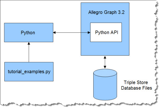
The Python client tutorial rests on a simple architecture involving AllegroGraph, disk-based data files, Python, and a file of Python examples called tutorial_examples.py.

AllegroGraph 3.2 Server runs as a Windows service in this example. It contains the Python API, which is part of the AllegroGraph installation. Python communicates with AllegroGraph through HTTP port 8080 in this example. Python and AllegroGraph may be installed on the same computer, but in practice one server is shared by multiple clients. Load tutorial_examples.py into Python to view the tutorial examples.

Each lesson in tutorial_examples.py is encapsulated in a Python function, named testN(), where N ranges from 0 to 19 (or more). The function names are referenced in the title of each section to make it easier to compare the tutorial text and the living code of the examples file.

Prerequisites (Windows)    Return to Top

The tutorial examples can be run on a 32-bit Windows XP computer, running AllegroGraph and Python on the same computer ("localhost"). The tutorial assumes that AllegroGraph and Python 2.5 have been installed and configured using this procedure:

1. Download an AllegroGraph 3.2 installation file (agraph-3.2-windows.exe). The free edition is available here. For the licensed edition please contact Franz customer support for a download link and authorizing key.
2. Run the agraph-3.2-windows.exe to install AllegroGraph. The default installation directory is C:\Program Files\AllegroGraphFSE32 for the free edition, or c:\Program Files\AllegroGraphSEE32 for the licensed edition.
3. Create a scratch directory for AllegroGraph to use for disk-based data storage. In this tutorial the directory is c:\tmp\scratch. If you elect to use a different location, the configuration and example files will have to be modified in the same way.
4. Edit the agraph.cfg configuration file. You'll find it in the AllegroGraph installation directory. Set the following parameters to the indicated values.

   :new-http-port 8080
   :new-http-catalog ("c:/tmp/scratch")
   :client-prolog t 

   If you use a different port number, you will need to change the value of the AG_PORT variable at the top of tutorial_examples.py. It defaults to 8080.
   
   NOTE: On Windows Vista and Windows 7 systems, you must edit this file with elevated privileges. To do this, either start a Command Prompt with  the context menu item "Run as Administrator" then edit the file using a text editor launched in that shell, or run your favorite editor with "Run as Administrator". If you do not edit with elevated privileges, the file will look like it was saved successfully but the changes will not be seen by the service when it is started. This produces a "cannot connect to server" error message.
5. To update AllegroGraph Server with recent patches, open a connection to the Internet. Run updater.exe, which you will find the AllegroGraph installation directory. This automatically downloads and installs all current patches.
6. On a Windows computer, the AllegroGraph Server runs as a Windows service. You have to restart this service to load the updates. Beginning at the Windows Start button, navigate this path:
   
   Start > Settings > Control Panel > Administrative Tools > Services.
   
   Locate the AllegroGraph Server service and select it. Click the Restart link to restart the service.
7. This example used ActivePython 2.5 from ActiveState.com. Download and install the Windows installation file, ActivePython-2.5.2.2-win32-x86.msi. The default installation direction is C:\Python25.
8. It is necessary to augment Python 2.5 with the CJSON package from python.cs.hu. Download and run the installation file, python-cjson-1.0.3x6.win32-py2.5.exe. It will add files to the default Python directory structure.
9. It is also necessary to augment Python 2.5 with the Pycurl package. Download and run the installation file, pycurl-ssl-7.18.2.win32-py2.5.exe. It will add a small directory to your default Python directory structure.
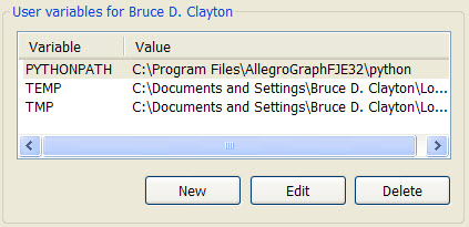
10. Link the Python software to the AllegroGraph Python API by setting a PYTHONPATH environment variable. For the free edition of AllegroGraph, the path value is:

    PYTHONPATH=C:\Program Files\AllegroGraphFSE32\python

    For the licensed edition of AllegroGraph, the path value is:

    PYTHONPATH=C:\Program Files\AllegroGraphSEE32\python

    In Windows XP, you can set an environment variable by right-clicking on the My Computer icon, then navigate to Properties > Advanced tab > Environment Variables. Create a new variable showing the path to the AllegroGraph python subdirectory.
    
    
    
11. Start the ActivePython 2.5 PythonWin editor. Navigate this path: Start button > Programs > ActiveState ActivePython 2.5 > PythonWin Editor.
12. In the PythonWin editor, open the File menu, select Run, and browse to the location of the tutorial_examples.py file. It will be in the AllegroGraph\python subdirectory. Run this file. This loads and runs the Python tutorial examples.

Prerequisites (Linux)   Return to Top

The tutorial examples can be run on a Linux system, running AllegroGraph and Python on the same computer ("localhost"). The tutorial assumes that AllegroGraph and Python 2.5 have been installed and configured using this procedure:

1. There are two Linux versions of AllegroGraph: 32-bit (x86) and 64-bit (x86-64). This example uses the 64-bit version. AllegroGraph is distributed both as an RPM and a tar.gz file. This example uses the RPM file.  Download the appropriate AllegroGraph Free Server Edition as directed by Franz customer support. In this example, the file was agraph-3.2-1.x86_64.rpm.
2. Use the Red Hat Package Manager (RPM) to install the AllegroGraph package.

   # rpm -i agraph-3.2-1.x86_64.rpm
   

3. Set up AllegroGraph as a service that runs automatically at startup.

   # chkconfig --add agraph

4. Start the AllegroGraph service.
   

   # service agraph start

5. Edit the agraph.cfg configuration file. You'll find it in the agraph-fse-3.2 subdirectory.  The rpm's default
       location for this subdirectory is "/usr/lib/agraph-fse-3.2". Set the following parameters to the indicated values.

          :new-http-port 8080
          :new-http-catalog ("/tmp/scratch")
          :client-prolog t

6. You'll have to restart the AllegroGraph Server to force it to load the edited configuration file.
   

   # service agraph restart

7. If Python is not pre-installed on your Linux system, you'll have to download and install it as a module. See the Python download page.
8. AllegroGraph requires the Python cjson and pycurl libraries. Please see your distributions documentation on how to install these libraries.  On a redhat-based distribution you can use the following:
   

   # yum install python-cjson python-pycurl

   or on a debian based system:
   

   # apt-get install python-cjson python-pycurl

   If your distribution does not offer these libraries then installation from source is recommended.
9. To test the installation, navigate to the /agraph-fse-3.2/python/ directory and run the tutorial file.
   

   # python tutorial_examples.py

   The command window will fill with output from the example functions described below.

Terminology   Return to Top

We need to clarify some terminology before proceeding.

• "RDF" is the Resource Description Framework defined by the World Wide Web Consortium (W3C). It provides a elegantly simple means for describing multi-faceted resource objects and for linking them into complex relationship graphs. AllegroGraph Server creates, searches, and manages such RDF graphs.
• A "URI" is a Uniform Resource Identifier. It is label used to uniquely identify variosu types of entities in an RDF graph. A typical URI looks a lot like a web address: <http:\\www.company.com\project\class#number>. In spite of the resemblance, a URI is not a web address. It is simply a unique label.
• A "triple" is a data statement, a "fact," stored in RDF format. It states that a resource has an attribute with a value. It consists of three fields:
• Subject: The first field contains the URI that uniquely identifies the resource that this triple describes.
• Predicate: The second field contains the URI identifying a property of this resource, such as its color or size, or a relationship between this resource and another one, such as parentage or ownership.
• Object: The third field is the value of the property. It could be a literal value, such as "red," or the URI of a linked resource.
• A "quad" is a triple with an added "context" field, which is used to divide the repository into "subgraphs." This context or subgraph is just a URI label that appears in the fourth field of related triples.
• A "quint" is a quad with fifth field used for the "tripleID." AllegroGraph Server implements all triples as quints behind the scenes. The fourth and fifth fields are often ignored, however, so we speak casually of "triples," and sometimes of "quads," when it would be more rigorous to call them all "quints."
• A "resource description " is defined as a collection of triples that all have the same URI in the subject field. In other words, the triples all describe attributes of the same thing.
• A "statement" is a client-side Python object that describes a triple (quad, quint). 

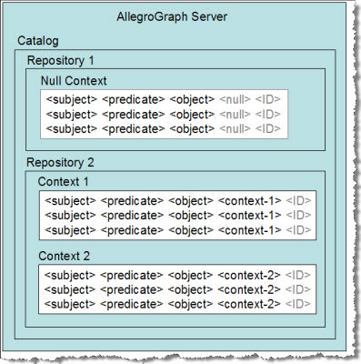
In the context of AllegroGraph Server: A "catalog" is a list of repositories owned by an AllegroGraph server. A "repository" is a collection of triples within a Catalog, stored and indexed on a hard disk. A "context" is a subgraph of the triples in a repository. If contexts are not in use, the triples are stored in the "null" context. If contexts are being used, the "null" context is not available.

Creating a Repository (test1())    Return to Top

The first task is to our AllegroGraph Server and open a repository. This task is implemented in test1() from tutorial_examples.py.

In test1() we build a chain of Python objects, ending in a"connection" object that lets us manipulate triples in a specific repository. The overall process of generating the connection object follows this diagram:

The test1() function opens (or creates) a repository by building a series of client-side objects, culminating in a "connection" object. The connection object will be passed to other functions in tutorial_examples.py. The connection object contains the methods that let us manipulate triples in a specific repository.

The example first connects to an AllegroGraph Server by providing the endpoint (host IP address and port number) of an already-launched AllegroGraph server. This creates a client-side server object, which can access the AllegroGraph server's list of available catalogs through the listCatalogs() method:.

def test1(accessMode=Repository.RENEW):
    server = AllegroGraphServer(path="localhost", port="8080")
    print "Available catalogs", server.listCatalogs()

This is the output so far:

>>> test1()
Defining connnection to AllegroGraph server -- host:'localhost' port:8080
Available catalogs ['scratch']

In the next line of test1(), we use the openCatalog() method to create a client-side catalog object. This object has methods such as getName() and listRepositories() that we can use to investigate the catalogs on the AllegroGraph server.. When we look inside the "scratch" catalog, we can see which repositories are available:

    catalog = server.openCatalog('scratch') 
    print "Available repositories in catalog '%s': %s" % (catalog.getName(), catalog.listRepositories()) 

The corresponding output lists the available repositories. (When you run the examples, you may see a different list of repositories.)

Available repositories in catalog 'scratch': ['agraph_test', 'greenthings', 'redthings', 'rainbowthings']  

The next step is to create a client-side repository object representing the respository we wish to open, by calling the getRepository() method of the catalog object. We have to provide the name of the desired repository (agraph_test in this case), and select one of four access modes:

• Repository.RENEW clears the contents of an existing repository before opening. If the indicated repository does not exist, it creates one.
• Repository.OPEN opens an existing repository, or throws an exception if the repository is not found.
• Repository.ACCESS opens an existing repository, or creates a new one if the repository is not found.
• Repository.CREATE creates a new repository, or throws an exception if one by that name already exists.

Repository.RENEW is the default setting for the test1() function of tutorial_examples.py. It can be overridden by calling test1() with the appropriate argument, such as test1(Repository.OPEN).

    myRepository = catalog.getRepository("agraph_test", accessMode)
    myRepository.initialize()

A new or renewed repository must be initialized, using the initialize() method of the repository object. If you try to initialize a respository twice you get a warning message in the Python window but no exception.

The goal of all this object-building has been to create a client-side connection object, whose methods let us manipulate the triples of the repository. The repository object's getConnection() method returns this connection object.

    connection = myRepository.getConnection()
    print "Repository %s is up! It contains %i statements." % (
    myRepository.getDatabaseName(), connection.size())
    return connection

The size() method of the connection object returns how many triples are present. In the test1() function, this number should always be zero because we "renewed" the repository. This is the output in the Python window:

   Repository agraph_test is up! It contains 0 statements.
   <franz.openrdf.repository.repositoryconnection.RepositoryConnection object at 0x0127D710>
 >>> 

The last line is the pointer to the new connection object. This is the value returned by test1() when it is called by other functions in tutorial_examples.py. The other functions then use the connection object to access the repository.

Asserting and Retracting Triples (test2())    Return to Top

In example test2(), we show how to create resources describing two people, Bob and Alice, by asserting individual triples into the respository. The example also retracts and replaces a triple. Assertions and retractions to the triple store are executed by 'add' and 'remove' methods belonging to the connection object, which we obtain by calling the test1() function (described above).

Before asserting a triple, we have to generate the URI values for the subject, predicate and object fields. The Python API to AllegroGraph Server predefines a number of classes and predicates for the RDF, RDFS, XSD, and OWL ontologies. RDF.TYPE is one of the predefined predicates we will use.

The 'add' and 'remove' methods take an optional 'contexts' argument that specifies one or more contexts that are the target of triple assertions and retractions. When the context is omitted, triples are asserted/retracted to/from the null context. In the example below, facts about Alice and Bob reside in the null context.

The test2() function begins by calling test1() to create the appropriate connection object, which is bound to the variable conn.

def test2():
    conn = test1()

The next step is to begin assembling the URIs we will need for the new triples. The createURI() method generates a URI from a string. These are the subject URIs identifying the resources "Bob" and "Alice":

    alice = conn.createURI("http://example.org/people/alice")
    bob = conn.createURI("http://example.org/people/bob")

Bob and Alice will be members of the "person" class (RDF:TYPE person).

    person = conn.createURI("http://example.org/ontology/Person")

Both Bob and Alice will have a "name" attribute.

    name = conn.createURI("http://example.org/ontology/name")

The name attributes will contain literal values. We have to generate the Literal objects from strings:

    bobsName = conn.createLiteral("Bob")
    alicesName = conn.createLiteral("Alice")

The next line prints out the number of triples currently in the repository.

    print "Triple count before inserts: ", conn.size()

Triple count before inserts:  0

Now we assert four triples, two for Bob and two more for Alice, using the connection object's add() method. After the assertions, we count triples again (there should be four) and print out the triples for inspection.

    ## alice is a person
    conn.add(alice, RDF.TYPE, person)
    ## alice's name is "Alice"
    conn.add(alice, name, alicesName)
    ## bob is a person
    conn.add(bob, RDF.TYPE, person)
    ## bob's name is "Bob":
    conn.add(bob, name, bobsName)

    print "Triple count: ", conn.size()
    for s in conn.getStatements(None, None, None, None): print s 

The "None" arguments to the getStatements() method say that we don't care what values are present in the subject, predicate, object or context positions. Just print out all the triples.

This is the output at this point. We see four triples, two about Alice and two about Bob:

Triple count:  4
(<http://example.org/people/alice>, <http://www.w3.org/1999/02/22-rdf-syntax-ns#type>, <http://example.org/ontology/Person>)
(<http://example.org/people/alice>, <http://example.org/ontology/name>, "Alice")
(<http://example.org/people/bob>, <http://www.w3.org/1999/02/22-rdf-syntax-ns#type>, <http://example.org/ontology/Person>)
(<http://example.org/people/bob>, <http://example.org/ontology/name>, "Bob")

We see two resources of type "person," each with a literal name.

The next step is to demonstrate how to remove a triple. Use the remove() method of the connection object, and supply a triple pattern that matches the target triple. In this case we want to remove Bob's name triple from the repository. Then we'll count the triples again to verify that there are only three remaining. Finally, we re-assert Bob's name so we can use it in subsequent examples, and we'll return the connection object..

    conn.remove(bob, name, bobsName)
    print "Triple count: ", conn.size()
    conn.add(bob, name, bobsName)    
    return conn

Triple count:  3
<franz.openrdf.repository.repositoryconnection.RepositoryConnection object at 0x01466830>

A SPARQL Query (test3())    Return to Top

SPARQL stands for the "SPARQL Protocol and RDF Query Language," a recommendation of the World Wide Web Consortium (W3C). SPARQL is a query language for retrieving RDF triples.

Our next example illustrates how to evaluate a SPARQL query. This is the simplest query, the one that returns all triples. Note that test3() continues with the four triples created in test2().

def test3():    
    conn = test2()
    try:
        queryString = "SELECT ?s ?p ?o  WHERE {?s ?p ?o .}"

The SELECT clause returns the variables ?s, ?p and ?o in the bindingSet. The variables are bound to the subject, predicate and objects values of each triple that satisfies the WHERE clause. In this case the WHERE clause is unconstrained. The dot (.) in the fourth position signifies the end of the pattern.

The connection object's prepareTupleQuery() method creates a query object that can be evaluated one or more times. (A "tuple" is an ordered sequence of data elements in Python.) The results are returned in an iterator that yields a sequence of bindingSets.

        tupleQuery = conn.prepareTupleQuery(QueryLanguage.SPARQL, queryString)
        result = tupleQuery.evaluate();

Below we illustrate one (rather heavyweight) method for extracting the values from a binding set, indexed by the name of the corresponding column variable in the SELECT clause.

        try:
            for bindingSet in result:
                s = bindingSet.getValue("s")
                p = bindingSet.getValue("p")
                o = bindingSet.getValue("o")              
                print "%s %s %s" % (s, p, o)

http://example.org/people/alice http://www.w3.org/1999/02/22-rdf-syntax-ns#type http://example.org/ontology/Person
http://example.org/people/alice http://example.org/ontology/name "Alice"
http://example.org/people/bob http://www.w3.org/1999/02/22-rdf-syntax-ns#type http://example.org/ontology/Person
http://example.org/people/bob http://example.org/ontology/name "Bob"

The Connection class is designed to be created for the duration of a sequence of updates and queries, and then closed. In practice, many AllegroGraph applications keep a connection open indefinitely. However, best practice dictates that the connection should be closed, as illustrated below. The same hygiene applies to the iterators that generate binding sets.

        finally:
            result.close();
    finally:
        conn.close();

Statement Matching (test4())    Return to Top

The getStatements() method of the connection object provides a simple way to perform unsophisticated queries. This method lets you enter a mix of required values and wildcards, and retrieve all matching triples. (If you need to perform sophisticated tests and comparisons you should use the SPARQL query instead.)

Below, we illustrate two kinds of 'getStatement' calls. The first mimics traditional Sesame syntax, and returns a Statement object at each iteration. This is the test4() function of tutorial_examples.py. It begins by calling test2() to create a connection object and populate the agraph_test repository with four triples describing Bob and Alice. We're going to search for triples that mention Alice, so we have to create an "Alice" URI to use in the search pattern:

def test4():
    conn = test2()
    alice = conn.createURI("http://example.org/people/alice")

Now we search for triples with Alice's URI in the subject position. The "None" values are wildcards for the predicate and object positions of the triple.

    print "Searching for Alice using getStatements():"
    statements = conn.getStatements(alice, None, None)

The getStatements() method returns a repositoryResult object (bound to the variable "statements" in this case). This object can be iterated over, exposing one result statement at a time. It is sometimes desirable to screen the results for duplicates, using the enableDuplicateFilter() method. Note, however, that duplicate filtering can be expensive. Our example does not contain any duplicates, but it is possible for them to occur.

    statements.enableDuplicateFilter() 
    for s in statements:
        print s

This prints out the two matching triples for "Alice."

Searching for Alice using getStatements():
(<http://example.org/people/alice>, <http://www.w3.org/1999/02/22-rdf-syntax-ns#type>, <http://example.org/ontology/Person>)
(<http://example.org/people/alice>, <http://example.org/ontology/name>, "Alice") 

At this point it is good form to close the respositoryResponse object because they occupy memory and are rarely reused in most programs.

	statements.close()

The test4() example continues with a second, more efficient way to perform simple retrievals. The second syntax borrows a trick from the JDBC API commonly used to access relational databases. The getJDBCStatements() method returns a ResultSet object that lets us iterate over the returned triples. A resultSet iterator does not materialize objects unless forced to. In this example it materializes only the object values of the returned triples. The getValue() method forces materialization of a resource or literal as an object, while the getString() call returns a string without creating an object. Developers who care about minimizing garbage will prefer to use the getJDBCStatements()' call, and they will usually call getString() in preference to getValue().

    print "Same thing using JDBC:"
    resultSet = conn.getJDBCStatements(alice, None, None)
    while resultSet.next():        
        print "   ", resultSet.getValue(2), "   ", resultSet.getString(2)  

The output is:

Same thing using JDBC:
    http://example.org/ontology/Person http://example.org/ontology/Person
    "Alice"    Alice  

Literal Values (test5())   Return to Top

The next example, test5(), illustrates some variations on what we have seen so far. The example creates and asserts typed literal values, including language-specific literals.

First, test5() obtains a connection object from test1(), and then clears the repository of all existing triples.

def test5():
    conn = test1()
    conn.clear()

For sake of coding efficiency, it is good practice to create variables for namespace strings. We'll use this namespace again and again in the following lines.

    exns = "http://example.org/people/"

The example creates new resources describing Alice and Ted. Apparently Bob took the day off. These are URIs to use in the subject field of the triples.

    alice = conn.createURI("http://example.org/people/alice")
    ted = conn.createURI(namespace=exns, localname="Ted")

These are the URIs of the four predicates used in the example: age, weight, favoriteColor, and birthdate.

    age = conn.createURI(namespace=exns, localname="age")
    weight = conn.createURI(namespace=exns, localname="weight")    
    favoriteColor = conn.createURI(namespace=exns, localname="favoriteColor")
    birthdate = conn.createURI(namespace=exns, localname="birthdate")

Favorite colors, declared in English (default) and French.

    red = conn.createLiteral('Red')
    rouge = conn.createLiteral('Rouge', language="fr")

Age values, declared as INT, LONG, and untyped:

    fortyTwo = conn.createLiteral('42', datatype=XMLSchema.INT)
    fortyTwoInteger = conn.createLiteral('42', datatype=XMLSchema.LONG)    
    fortyTwoUntyped = conn.createLiteral('42')

Birth date values, declared as DATE and DATETIME types.

    date = conn.createLiteral('1984-12-06', datatype=XMLSchema.DATE)     
    time = conn.createLiteral('1984-12-06T09:00:00', datatype=XMLSchema.DATETIME) 

Weights, written as floats, but one untyped and the other declared to be a FLOAT.

    weightFloat = conn.createLiteral('20.5', datatype=XMLSchema.FLOAT)
    weightUntyped = conn.createLiteral('20.5') 

The connection object's createStatement() method assembles the elements of a triple, but does not yet add them to the repository. Here are Alice's and Ted's ages assembled into statements:

    stmt1 = conn.createStatement(alice, age, fortyTwo)
    stmt2 = conn.createStatement(ted, age, fortyTwoUntyped)  

The Python API to AllegroGraph Server offers add(), addStatement(), addFile(), addTriple(), and addTriples() methods for asserting triples into the repository. (There is substantial overlap among these methods becuase the Python API attempts to be compatible other, similar APIs.) Below, we show add(), addStatement(), addTriple(), and addTriples() calls side-by-side. The demonstration of addFiles() is in the next example. Best practice would be to used addTriples() and addFile() in most situations.

    conn.add(stmt1)
    conn.addStatement(stmt2)
    conn.addTriple(alice, weight, weightUntyped)
    conn.addTriple(ted, weight, weightFloat)
    conn.addTriples([(alice, favoriteColor, red),
                     (ted, favoriteColor, rouge),
                     (alice, birthdate, date),
                     (ted, birthdate, time)])

The RDF/SPARQL spec is very conservative when matching various combinations of literal values. The match and query statements below illustrate how some of these combinations perform. Note that this loop uses the getStatements() method to retrieve triples.

    for obj in [None, fortyTwo, fortyTwoUntyped, conn.createLiteral('20.5', 
                datatype=XMLSchema.FLOAT), conn.createLiteral('20.5'), red, rouge]:
        print "Retrieve triples matching '%s'." % obj
        statements = conn.getStatements(None, None, obj)
        for s in statements:
            print s

These are the results of the tests in this loop:

Retrieve triples matching 'None'. ['None' matches all values of all types.]
(<http://example.org/people/alice>, <http://example.org/people/age>, "42"^^<http://www.w3.org/2001/XMLSchema#int>)
(<http://example.org/people/Ted>, <http://example.org/people/age>, "42")
(<http://example.org/people/alice>, <http://example.org/people/weight>, "20.5")
(<http://example.org/people/Ted>, <http://example.org/people/weight>, "20.5"^^<http://www.w3.org/2001/XMLSchema#float>)
(<http://example.org/people/alice>, <http://example.org/people/favoriteColor>, "Red")
(<http://example.org/people/Ted>, <http://example.org/people/favoriteColor>, "Rouge"@fr)
(<http://example.org/people/alice>, <http://example.org/people/birthdate>, "1984-12-06"^^<http://www.w3.org/2001/XMLSchema#date>)
(<http://example.org/people/Ted>, <http://example.org/people/birthdate>, "1984-12-06T09:00:00"^^<http://www.w3.org/2001/XMLSchema#dateTime>)

Retrieve triples matching '"42"^^<http://www.w3.org/2001/XMLSchema#int>'. [INT matches only the INT triple.]
   (<http://example.org/people/alice>, <http://example.org/people/age>, "42"^^<http://www.w3.org/2001/XMLSchema#int>)
   
Retrieve triples matching '"42"'.  [String matches string.]
   (<http://example.org/people/Ted>, <http://example.org/people/age>, "42")   

Retrieve triples matching '"20.5"^^<http://www.w3.org/2001/XMLSchema#float>'. [FLOAT matches FLOAT.]
   (<http://example.org/people/Ted>, <http://example.org/people/weight>, "20.5"^^<http://www.w3.org/2001/XMLSchema#float>)   

Retrieve triples matching '"20.5"'. [String matches string, but not FLOAT.]
   (<http://example.org/people/alice>, <http://example.org/people/weight>, "20.5")   

Retrieve triples matching '"Red"'.  [String matches string.]
   (<http://example.org/people/alice>, <http://example.org/people/favoriteColor>, "Red")   

Retrieve triples matching '"Rouge"@fr'. [French string matches French string.]
   (<http://example.org/people/Ted>, <http://example.org/people/favoriteColor>, "Rouge"@fr)   

This second loop illustrates an alternate syntax for pulling values out of a BindingSet object which takes advantage of the fact that our BindingSet can emulate a Python 'dict'. This loop builds and evaluates a SPARQL query instead of using getStatements().

    for obj in ['42', '"42"', '20.5', '"20.5"', '"20.5"^^xsd:float', '"Rouge"@fr', '"Rouge"', 
                '"1984-12-06"^^xsd:date']:
        print "Query triples matching '%s'." % obj
        queryString = """PREFIX xsd: <http://www.w3.org/2001/XMLSchema#> 
        SELECT ?s ?p ?o WHERE {?s ?p ?o . filter (?o = %s)}
        """ % obj
        tupleQuery = conn.prepareTupleQuery(QueryLanguage.SPARQL, queryString)
        result = tupleQuery.evaluate();    
        for bindingSet in result:
            s = bindingSet[0]
            p = bindingSet[1]
            o = bindingSet[2]
            print "%s %s %s" % (s, p, o)

These are the results of this loop:

Query triples matching '42'. [INT matches INT.]
http://example.org/people/alice http://example.org/people/age "42"^^<<http://www.w3.org/2001/XMLSchema#int>>
Query triples matching '"42"'. [String matches string.]
  http://example.org/people/Ted http://example.org/people/age "42"
Query triples matching '20.5'. [Float matches float.]
  http://example.org/people/Ted http://example.org/people/weight "20.5"^^<<http://www.w3.org/2001/XMLSchema#float>>
Query triples matching '"20.5"'.  [String matches string.]
  http://example.org/people/alice http://example.org/people/weight "20.5"
Query triples matching '"20.5"^^xsd:float'. [Float matches float.]
  http://example.org/people/Ted http://example.org/people/weight "20.5"^^<<http://www.w3.org/2001/XMLSchema#float>>
Query triples matching '"Rouge"@fr'.  [French string matches French string.]
  http://example.org/people/Ted http://example.org/people/favoriteColor "Rouge"@fr
Query triples matching '"Rouge"'. [General string fails to match French string.]

In the following example, we use getStatements() to match a DATE object:

    ## Search for date using date object in triple pattern.
    print "Retrieve triples matching DATE object."
    statements = conn.getStatements(None, None, date)
    for s in statements:
        print s

Retrieve triples matching DATE object.
(<http://example.org/people/alice>, <http://example.org/people/birthdate>, 
"1984-12-06"^^<http://www.w3.org/2001/XMLSchema#date>)

Note the string representation of the DATE object. We can plug that into a query as a string to make the same match:

    print "Match triples having a specific DATE value."
    statements = conn.getStatements(None, None, '"1984-12-06"^^<http://www.w3.org/2001/XMLSchema#date>')
    for s in statements:
        print s

Match triples having specific DATE value.
(<http://example.org/people/alice>, <http://example.org/people/birthdate>, "1984-12-06"^^<http://www.w3.org/2001/XMLSchema#date>)

Importing Triples (test6() and test7())    Return to Top

The Python API client can load triples in either RDF/XML format or NTriples format. The example below calls the connection object's add() method to load an NTriples file, and addFile() to load an RDF/XML file. Both methods work, but the best practice is to use addFile().

The RDF/XML file contains a short list of v-cards (virtual business cards), like this one:

  <rdf:Description rdf:about="http://somewhere/JohnSmith/">
    <vCard:FN>John Smith</vCard:FN>
    <vCard:N rdf:parseType="Resource">
	    <vCard:Family>Smith</vCard:Family>
	    <vCard:Given>John</vCard:Given>
    </vCard:N>
  </rdf:Description> 

The NTriples file contains a graph of resources describing the Kennedy family, the places where they were each born, their colleges, and their professions. A typical entry from that file looks like this:

<http://www.franz.com/simple#person1> <http://www.franz.com/simple#first-name> "Joseph" . 
<http://www.franz.com/simple#person1> <http://www.franz.com/simple#middle-initial> "Patrick" . 
<http://www.franz.com/simple#person1> <http://www.franz.com/simple#last-name> "Kennedy" . 
<http://www.franz.com/simple#person1> <http://www.franz.com/simple#suffix> "none" . 
<http://www.franz.com/simple#person1> <http://www.franz.com/simple#alma-mater> <http://www.franz.com/simple#Harvard> . 
<http://www.franz.com/simple#person1> <http://www.franz.com/simple#birth-year> "1888" . 
<http://www.franz.com/simple#person1> <http://www.franz.com/simple#death-year> "1969" . 
<http://www.franz.com/simple#person1> <http://www.franz.com/simple#sex> <http://www.franz.com/simple#male> . 
<http://www.franz.com/simple#person1> <http://www.franz.com/simple#spouse> <http://www.franz.com/simple#person2> . 
<http://www.franz.com/simple#person1> <http://www.franz.com/simple#has-child> <http://www.franz.com/simple#person3> . 
<http://www.franz.com/simple#person1> <http://www.franz.com/simple#profession> <http://www.franz.com/simple#banker> . 
<http://www.franz.com/simple#person1> <http://www.franz.com/simple#birth-place> <http://www.franz.com/simple#place5> . 
<http://www.franz.com/simple#person1> <http://www.w3.org/1999/02/22-rdf-syntax-ns#type> <http://www.franz.com/simple#person> . 

Note that AllegroGraph can segregate triples into contexts by treating them as quads, but the NTriples and RDF/XML formats can not include contexts. They deal with triples only. In the case of the add() call, we have omitted the context argument so the triples are loaded by default into the null context. The addFile() call includes an explicit context setting, so the fourth argument of each vcard triple will be the context named "/tutorial/vc_db_1_rdf". The connection size() method takes an optional context argument. With no argument, it returns the total number of triples in the repository. Below, it returns the number '16' for the 'context' context argument, and the number '28' for the null context (None) argument.

The test6() function of tutorial_examples.py obtains a connection object from test1(), and then clears out the existing triples.

def test6():
    conn = test1()
    conn.clear()   

The variables path1 and path2 are bound to the RDF/XML and NTriples files, respectively.

    path1 = "./vc-db-1.rdf"    
    path2 = "./kennedy.ntriples"                

Both examples need a base URI as one of the required arguments to the asserting methods:

    baseURI = "http://example.org/example/local"

The NTriples about the Kennedy family will be added to a specific context, so naturally we need a URI to identify that context.

    context = conn.createURI("http://example.org#vcards")

In the next step, we use add() to load the Kennedy family tree into the null context:

    conn.add(path2, base=baseURI, format=RDFFormat.NTRIPLES, contexts=None)

Then we use addFile() to load the vcard triples into the #vcards context:

    conn.addFile(path1, baseURI, format=RDFFormat.RDFXML, context=context);

Loading the triples does not index them. Whenever a significant number of updates is made to the RDF store, the method indexTriples() should be called. In this example, it is called after both files have been loaded. The argument "all=True" tells it to (re)index all triples in the store. The default behavior is to only index triples updates since the last call to indexTriples(). In that case, indexing is quicker, but the data structures are not quite as well-organizezd.

    conn.indexTriples(all=True)

Now we'll ask AllegroGraph to report on how many triples it sees in the null context and in the #vcards context:

    print "After loading, repository contains %i vcard triples in context '%s'\n    
           and   %i kennedy triples in context '%s'." % 
           (conn.size(context), context, conn.size('null'), 'null')
    return conn

The output of this report was:

After loading, repository contains 16 vcard triples in context 'http://example.org#vcards'
    and   1214 kennedy triples in context 'null'. 

The SPARQL query below is found in test7() of tutorial_examples.py. It borrows the same triples we loaded in test6(), above, and runs two unconstrained retrievals. The first uses getStatement, and prints out the subject URI and context of each triple.

def test7():    
    conn = test6()
    print "Match all and print subjects and contexts"
    result = conn.getStatements(None, None, None, None, limit=25)
    for row in result: print row.getSubject(), row.getContext()

This loop prints out a mix of triples from the null context and from the #vcards context. We set a limit of 25 triples because the Kennedy dataset contains over a thousand triples.

The following loop, however, does not produce the same results. This is a SPARQL query that should match all available triples, printout out the subject and context of each triple:

    print "\nSame thing with SPARQL query (can't retrieve triples in the null context)"
    queryString = "SELECT DISTINCT ?s ?c WHERE {graph ?c {?s ?p ?o .} }"
    tupleQuery = conn.prepareTupleQuery(QueryLanguage.SPARQL, queryString)
    result = tupleQuery.evaluate();
    for i, bindingSet in enumerate(result):
        print bindingSet[0], bindingSet[1]
    conn.close()

In this case, the loop prints out only eight triples. These are the eight from the #vcards context. The SPARQL query is not able to access the null context.

Exporting Triples (test8() and test9())    Return to Top

The next examples show how to write triples out to a file in either NTriples format or RDF/XML format. The output of either format may be optionally redirected to standard output (the Python command window) for inspection.

Example test8() begins by obtaining a connection object from test6(). This means the repository contains v-card triples in the #vcards context, and Kennedy family tree triples in the null context.

def test8():
    conn = test6()

In this example, we'll export the triples in the #vcards context.

    context = conn.createURI("http://example.org#vcards")

To write triples in NTriples format, call NTriplesWriter(). You have to tell it the path and file name of the exported file. If the output file argument is 'None', the writers write to standard output. You can uncomment that line if you'd like to see it work.

    outputFile = "/tmp/temp.nt"
    #outputFile = None
    if outputFile == None:
        print "Writing RDF to Standard Out instead of to a file"
    ntriplesWriter = NTriplesWriter(outputFile)
    conn.export(ntriplesWriter, context);

To write triples in RDF/XML format, call RDFXMLWriter().

    outputFile2 = "/tmp/temp.rdf"
    #outputFile2 = None
    if outputFile2 == None:
        print "Writing NTriples to Standard Out instead of to a file"
    rdfxmlfWriter = RDFXMLWriter(outputFile2)    
    conn.export(rdfxmlfWriter, context)

The export() method writes out all triples in one or more contexts. This provides a convenient means for making local backups of sections of your RDF store. If two or more contexts are specified, then triples from all of those contexts will be written to the same file. Since the triples are "mixed together" in the file, the context information is not recoverable. If the context argument is omitted, all triples in the store are written out, and again all context information is lost.

Finally, if the objective is to write out a filtered set of triples, the exportStatements() method can be used. The example below (from test9()) writes out all RDF:TYPE declaration triples to standard output.

conn.exportStatements(None, RDF.TYPE, None, False, RDFXMLWriter(None))

Datasets and Contexts (test10())    Return to Top

We have already seen contexts at work when loading and saving files. In test10() we provide more realistic examples of contexts, and we introduce the dataset object. A dataset is a list of contexts that should all be searched simultaneously.

To set up the example, we create six statements, and add two of each to three different contexts: context1, context2, and the null context.

conn.clear()
exns = "http://example.org/people/"
alice = f.createURI(namespace=exns, localname="alice")
bob = f.createURI(namespace=exns, localname="bob")
ted = f.createURI(namespace=exns, localname="ted")
person = f.createURI(namespace=exns, localname="Person")
name = f.createURI(namespace=exns, localname="name")    
alicesName = f.createLiteral("Alice")    
bobsName = f.createLiteral("Bob")
tedsName = f.createLiteral("Ted")    
context1 = f.createURI(namespace=exns, localname="cxt1")      
context2 = f.createURI(namespace=exns, localname="cxt2")          
conn.add(alice, RDF.TYPE, person, context1)
conn.add(alice, name, alicesName, context1)
conn.add(bob, RDF.TYPE, person, context2)
conn.add(bob, name, bobsName, context2)
conn.add(ted, RDF.TYPE, person)
conn.add(ted, name, tedsName)

The first test uses getStatements() to return all triples in all contexts (cxt1, cxt2, and null).

statements = conn.getStatements(None, None, None, False)
print "All triples in all contexts:"
for s in statements:
    print s

The output of this loop is shows below. The context URIs are in the fourth position. Triples from the null context have no context value.

All triples in all contexts:
(<http://example.org/people/alice>, <http://www.w3.org/1999/02/22-rdf-syntax-ns#type>, <http://example.org/people/Person>, <http://example.org/people/cxt1>)
(<http://example.org/people/alice>, <http://example.org/people/name>, "Alice", <http://example.org/people/cxt1>)
(<http://example.org/people/bob>, <http://www.w3.org/1999/02/22-rdf-syntax-ns#type>, <http://example.org/people/Person>, <http://example.org/people/cxt2>)
(<http://example.org/people/bob>, <http://example.org/people/name>, "Bob", <http://example.org/people/cxt2>)
(<http://example.org/people/ted>, <http://www.w3.org/1999/02/22-rdf-syntax-ns#type>, <http://example.org/people/Person>)
(<http://example.org/people/ted>, <http://example.org/people/name>, "Ted")

The next match explicitly lists 'context1' and 'context2' as the only contexts to participate in the match. It returns four statements.

statements = conn.getStatements(None, None, None, False, [context1, context2])
print "Triples in contexts 1 and 2:"
for s in statements:
    print s

The output of this loop shows that the triples in the null context have been excluded.

Triples in contexts 1 or 2:
(<http://example.org/people/alice>, <http://www.w3.org/1999/02/22-rdf-syntax-ns#type>, <http://example.org/people/Person>, <http://example.org/people/cxt1>)
(<http://example.org/people/alice>, <http://example.org/people/name>, "Alice", <http://example.org/people/cxt1>)
(<http://example.org/people/bob>, <http://www.w3.org/1999/02/22-rdf-syntax-ns#type>, <http://example.org/people/Person>, <http://example.org/people/cxt2>)
(<http://example.org/people/bob>, <http://example.org/people/name>, "Bob", <http://example.org/people/cxt2>)

This time we use getStatements() to search explicitly for triples in the null context and in context 2.

statements = conn.getStatements(None, None, None, ['null', context2])
print "Triples in contexts null or 2:"
for s in statements:
    print s

The output of this loop is:

Triples in contexts null or 2:
(<http://example.org/people/ted>, <http://www.w3.org/1999/02/22-rdf-syntax-ns#type>, <http://example.org/people/Person>)
(<http://example.org/people/ted>, <http://example.org/people/name>, "Ted")
(<http://example.org/people/bob>, <http://www.w3.org/1999/02/22-rdf-syntax-ns#type>, <http://example.org/people/Person>, <http://example.org/people/cxt2>)
(<http://example.org/people/bob>, <http://example.org/people/name>, "Bob", <http://example.org/people/cxt2>)

Next, we switch to SPARQL queries. Named contexts may be included in the FROM and FROM-NAMED clauses in a SPARQL query. Below, we illustrate the procedural equivalent, which is to create a dataset object, add the contexts to that, and then to attach the dataset to the query object. The query is (again) restricted to only those statements in contexts 1 and 2.

queryString = """
SELECT ?s ?p ?o ?c
WHERE { GRAPH ?c {?s ?p ?o . } } 
"""
ds = Dataset()
ds.addNamedGraph(context1)
ds.addNamedGraph(context2)
tupleQuery = conn.prepareTupleQuery(QueryLanguage.SPARQL, queryString)
tupleQuery.setDataset(ds)
result = tupleQuery.evaluate();    
print "Query over contexts 1 and 2."
for bindingSet in result:
    print bindingSet.getRow()

The output of this loop contains four triples, as expected.

Query over contexts 1 and 2.
['<http://example.org/people/alice>', '<http://www.w3.org/1999/02/22-rdf-syntax-ns#type>', '<http://example.org/people/Person>', '<http://example.org/people/cxt1>']
['<http://example.org/people/alice>', '<http://example.org/people/name>', '"Alice"', '<http://example.org/people/cxt1>']
['<http://example.org/people/bob>', '<http://www.w3.org/1999/02/22-rdf-syntax-ns#type>', '<http://example.org/people/Person>', '<http://example.org/people/cxt2>']
['<http://example.org/people/bob>', '<http://example.org/people/name>', '"Bob"', '<http://example.org/people/cxt2>']

Currently, its not possible to combine the null context with other contexts in a SPARQL query. Below, we illustrate how to evaluate a query against only the null context.

queryString = """
SELECT ?s ?p ?o    
WHERE {?s ?p ?o . } 
"""
ds = Dataset()
ds.addDefaultGraph(None)
tupleQuery = conn.prepareTupleQuery(QueryLanguage.SPARQL, queryString)
tupleQuery.setDataset(ds)
result = tupleQuery.evaluate();    
print "Query over the null context."
for bindingSet in result:
    print bindingSet.getRow()

The output of this loop is:

Query over the null context.
['<http://example.org/people/ted>', '<http://www.w3.org/1999/02/22-rdf-syntax-ns#type>', '<http://example.org/people/Person>']
['<http://example.org/people/ted>', '<http://example.org/people/name>', '"Ted"']

Namespaces (test11())    Return to Top

A namespace is that portion of a URI that preceeds the last '#', '/', or ':' character, inclusive. The remainder of a URI is called the localname. For example, with respect to the URI "http://example.org/people/alice", the namespace is "http://example.org/people/" and the localname is "alice". When writing SPARQL queries, it is convenient to define prefixes or nicknames for the namespaces, so that abbreviated URIs can be specified. For example, if we define "ex" to be a nickname for "http://example.org/people/", then the string "ex:alice" is a recognized abbreviation for "http://example.org/people/alice". This abbreviation is called a qname.

In the SPARQL query in the example below, we see two qnames, "rdf:type" and "ex:alice". Ordinarily, we would expect to see "PREFIX" declarations in SPARQL that define namespaces for the "rdf" and "ex" nicknames. However, the Connection and Query machinery can do that job for you. The mapping of prefixes to namespaces includes the built-in prefixes RDF, RDFS, XSD, and OWL. Hence, we can write "rdf:type" in a SPARQL query, and the system already knows its meaning. In the case of the 'ex' prefix, we need to instruct it. The setNamespace() method of the connection object registers a new namespace. In the example below, we first register the 'ex' prefix, and then submit the SPARQL query. It is legal, although not recommended, to redefine the built-in prefixes RDF, etc..

The example test11() begins by borrowing a connection object from test1().

def test11():
    conn = test1()

We need a namespace string (bound to the variable exns) to use when generating the alice and person URIs.

    exns = "http://example.org/people/"
    alice = conn.createURI(namespace=exns, localname="alice")
    person = conn.createURI(namespace=exns, localname="Person")

Now we can assert Alice's RDF:TYPE triple. Then we have to remind AllegroGraph to index it.

    conn.add(alice, RDF.TYPE, person)
    conn.indexTriples(all=True, asynchronous=True)

Now we register the exns namespace with the connection object, so we can use it in a SPARQL query. The query looks for triples that have "rdf:type" in the predicate position, and "ex:Person" in the object position.

    conn.setNamespace('ex', exns)
    queryString = """
    SELECT ?s ?p ?o 
    WHERE { ?s ?p ?o . FILTER ((?p = rdf:type) && (?o = ex:Person) ) }
    """
    tupleQuery = conn.prepareTupleQuery(QueryLanguage.SPARQL, queryString)
    result = tupleQuery.evaluate();  
    print    
    for bindingSet in result:
        print bindingSet[0], bindingSet[1], bindingSet[2]

The output shows the single triple with its fully-expanded URIs. This demonstrates that the qnames in the SPARQL query successfully matched the fully-expanded URIs in the triple.

http://example.org/people/alice http://www.w3.org/1999/02/22-rdf-syntax-ns#type http://example.org/people/Person

It is worthwhile to briefly discuss performance here. In the current AllegroGraph system, queries run more efficiently if constants appear inside of the "where" portion of a query, rather than in the "filter" portion. For example, the SPARQL query below will evaluate more efficiently than the one in the above example. However, in this case, you have lost the ability to output the constants "http://www.w3.org/1999/02/22-rdf-syntax-ns#type" and "http://example.org/people/alice". Occasionally you may find it useful to output constants in the output of a 'select' clause; in general though, the above code snippet illustrates a query syntax that is discouraged.

SELECT ?s  
WHERE { ?s rdf:type ex:person } 

Free Text Search (test12())    Return to Top

It is common for users to build RDF applications that combine some form of "keyword search" with their queries. For example, a user might want to retrieve all triples for which the string "Alice" appears as a word within the third (object) argument to the triple. AllegroGraph provides a capability for including free text matching within a SPARQL query. It requires, however, that you register the predicates that will participate in text searches so they can be indexed.

The example test12() begins by borrowing the connection object from test1(). Then it creates a namespace string and registers the namespace with the connection object, as in the previous example.

def test12():
    conn = test1()
    exns = "http://example.org/people/"
    conn.setNamespace('ex', exns)

We have to register the predicates that will participate in text indexing. In the test12() example below, we have called the connection method registerFreeTextPredicate() to register the predicate "http://example.org/people/fullname" for text indexing. Generating the predicate's URI is a separate step.

    conn.registerFreeTextPredicate(namespace=exns, localname='fullname')
    fullname = conn.createURI(namespace=exns, localname="fullname")    

The next step is to create two new resources, "Alice1" named "Alice B. Toklas," and "book1" with the title "Alice in Wonderland." Notice that we did not register the book title predicate for text indexing.

    alice = conn.createURI(namespace=exns, localname="alice1")
    persontype = conn.createURI(namespace=exns, localname="Person")
    alicename = conn.createLiteral('Alice B. Toklas')
    book =  conn.createURI(namespace=exns, localname="book1")
    booktype = conn.createURI(namespace=exns, localname="Book")
    booktitle = conn.createURI(namespace=exns, localname="title")    
    wonderland = conn.createLiteral('Alice in Wonderland')

Clear the repository, so our new triples are the only ones available.

    conn.clear()    

Add the resource for the new person, Alice B. Toklas:

    conn.add(alice, RDF.TYPE, persontype)
    conn.add(alice, fullname, alicename)

Add the new book, Alice in Wonderland. Index the triples.

    conn.add(book, RDF.TYPE, booktype)    
    conn.add(book, booktitle, wonderland) 
    conn.indexTriples(all=True, asynchronous=True)

Now we set up the SPARQL query that looks for triples containing "Alice" in the object position.

The text match occurs through a "magic" predicate called fti:match. This is not an RDF "predicate" but a LISP "predicate," meaning that it behaves as a true/false test. This predicate has two arguments. One is the subject URI of the resources to search. The other is the string pattern to search for, such as "Alice". Only registered text predicates will be searched. Only full-word matches will be found.

    conn.setNamespace('ex', exns)
    queryString = """
    SELECT ?s ?p ?o
    WHERE { ?s ?p ?o . ?s fti:match 'Alice' . }
    """
    tupleQuery = conn.prepareTupleQuery(QueryLanguage.SPARQL, queryString)
    result = tupleQuery.evaluate(); 

There is no need to include a prefix declaration for the 'fti' nickname. That is because 'fti' included among the built-in namespace/nickname mappings in AllegroGraph.

When we execute our SPARQL query, it matches the "Alice" within the literal "Alice B. Toklas" because that literal occurs in a triple having the registered fullname predicate, but it does not match the "Alice" in the literal "Alice in Wonderland" because the booktitle predicate was not registered for text indexing. This query returns all triples of a resource that had a successful match in at least one object value.

    print "Found %i query results" % len(result)    
    count = 0
    for bindingSet in result:
        print bindingSet
        count += 1
        if count > 5: break

The output of this loop is:

Found 2 query results
{'p': 'http://www.w3.org/1999/02/22-rdf-syntax-ns#type', 's': 'http://example.org/people/alice1', 'o': 'http://example.org/people/Person'}
{'p': 'http://example.org/people/fullname', 's': 'http://example.org/people/alice1', 'o': '"Alice B. Toklas"'}

The text index supports simple wildcard queries. The asterisk (*) may be appended to the end of the pattern to indicate "any number of additional characters." For instance, this query looks for whole words that begin with "Ali":

    queryString = """
    SELECT ?s ?p ?o
    WHERE { ?s ?p ?o . ?s fti:match 'Ali*' . }
    """

It finds the same two triples as before.

There is also a single-character wildcard, the questionmark. You can add as many question marks as you need to the string pattern. This query looks for a five-letter word that has "l" in the second position, and "c" in the fourth position:

    queryString = """
    SELECT ?s ?p ?o
    WHERE { ?s ?p ?o . ?s fti:match '?l?c?' . }
    """

This query finds the same two triples as before.

This time we'll do something a little different. The free text indexing matches whole words only, even when using wildcards. What if you really need to match a substring in a word of unknown length. You can write a SPARQL query that performs a regex match against object values. This can be inefficient compared to indexed search, and the match is not confined to the registered free-text predicates. The following query looks for the substring "lic" in literal object values:

    queryString = """
    SELECT ?s ?p ?o
    WHERE { ?s ?p ?o . FILTER regex(?o, "lic") }
    """

This query returns two triples, but they are not quite the same as before:

Substring match for 'lic'
Found 2 query results
{'p': 'http://example.org/people/fullname', 's': 'http://example.org/people/alice1', 'o': '"Alice B. Toklas"'}
{'p': 'http://example.org/people/title', 's': 'http://example.org/people/book1', 'o': '"Alice in Wonderland"'} 

As you can see, the regex match found "lic" in "Alice in Wonderland," which was not a registered free-text predicate. It made this match by doing a string comparison against every object value in the triple store. Even though you can streamline the SPARQL query considerably by writing more restrictive patterns, this is still inherently less efficient than using the indexed approach.

Ask, Describe, and Construct Queries (test13())   Return to Top

SPARQL provides alternatives to the standard SELECT query. Example test13() exercises these alternatives to show how AllegroGraph Server handles them.

• SELECT: Returns all, or a subset of, the variables bound in a query pattern match.
• CONSTRUCT: Returns an RDF graph constructed by substituting variables in a set of triple templates.
• ASK: Returns a boolean indicating whether a query pattern matches or not.
• DESCRIBE: Returns an RDF graph that describes the resources found.

The example begins by borrowing a connection object from test2(). Then it registers two namespaces for use in the SPARQL queries.:

def test13():
    conn = test2()
    conn.setNamespace('ex', "http://example.org/people/")
    conn.setNamespace('ont', "http://example.org/ontology/")

The example begins with an unconstrained SELECT query so we can see what triples are available for matching.

    queryString = """select ?s ?p ?o where { ?s ?p ?o} """
    tupleQuery = conn.prepareTupleQuery(QueryLanguage.SPARQL, queryString)
    result = tupleQuery.evaluate();
    print "SELECT result"
    for r in result: print r     

SELECT result
{'p': 'http://www.w3.org/1999/02/22-rdf-syntax-ns#type', 's': 'http://example.org/people/alice', 'o': 'http://example.org/ontology/Person'}
{'p': 'http://example.org/ontology/name', 's': 'http://example.org/people/alice', 'o': '"Alice"'}
{'p': 'http://www.w3.org/1999/02/22-rdf-syntax-ns#type', 's': 'http://example.org/people/bob', 'o': 'http://example.org/ontology/Person'}
{'p': 'http://example.org/ontology/name', 's': 'http://example.org/people/bob', 'o': '"Bob"'}

The ASK query returns a Boolean, depending on whether the triple pattern matched any triples. In this case it looks for any ont:name triplecontaining the value "Alice." Note that the ASK query uses a different construction method than the SELECT query: prepareBooleanQuery().

    queryString = """ask { ?s ont:name "Alice" } """
    booleanQuery = conn.prepareBooleanQuery(QueryLanguage.SPARQL, queryString)
    result = booleanQuery.evaluate(); 
    print "Boolean result", result

The output of this loop is:

Boolean result True

The CONSTRUCT query contructs a statement object out of the matching values in the triple pattern. A "statement" is a client-side triple. Construction queries use prepareGraphQuery(). The point is that the query can bind variables from existing triples and then "construct" a new triple by recombining the values.

    queryString = """construct {?s ?p ?o} where { ?s ?p ?o . filter (?o = "Alice") } """
    constructQuery = conn.prepareGraphQuery(QueryLanguage.SPARQL, queryString)
    result = constructQuery.evaluate(); 
    for st in result:
        print "Construct result, S P O values in statement:", st.getSubject(), st.getPredicate(), st.getObject()

The output of this loop is below. It has created a statement from values found in the repository.

Construct result, S P O values in statement: http://example.org/people/alice http://example.org/ontology/name "Alice"

    queryString = """describe ?s where { ?s ?p ?o . filter (?o = "Alice") } """
    describeQuery = conn.prepareGraphQuery(QueryLanguage.SPARQL, queryString)
    result = describeQuery.evaluate(); 
    print "Describe result"
    for st in result: print st 

The output of this loop is:

Describe result
(<http://example.org/people/alice>, <http://www.w3.org/1999/02/22-rdf-syntax-ns#type>, <http://example.org/ontology/Person>)
(<http://example.org/people/alice>, <http://example.org/ontology/name>, "Alice")

Parametric Queries (test14())   Return to Top

The Python API to AllegroGraph Server lets you set up a SPARQL query and then fix the value of one of the query variables prior to matching the triples. This is more efficient than testing for the same value in the body of the query.

In test14() we set up two-triple resources for Bob and Alice, and then use an unconstrained SPARQL query to retrieve the triples. Normally this query would find all four triples, but by binding the subject value ahead of time, we can retrieve the "Bob" triples separately from the "Alice" triples.

The example begins by borrowing a connection object from test2(). This means there are already Bob and Alice resources in the repository. We do need to recreate the URIs for the two resources, however.

def test14():
    conn = test2()
    alice = conn.createURI("http://example.org/people/alice")
    bob = conn.createURI("http://example.org/people/bob")

The SPARQL query is the simple, unconstrained query that returns all triples. We use prepareTupleQuery() to create the query object.

    queryString = """select ?s ?p ?o where { ?s ?p ?o} """
    tupleQuery = conn.prepareTupleQuery(QueryLanguage.SPARQL, queryString)

Before evaluating the query, however, we'll use the query objects setBinding() method to assign Alice's URI to the "s" variable in the query. This means that all matching triples are required to have Alice's URI in the subject position of the triple.

    tupleQuery.setBinding("s", alice)
    result = tupleQuery.evaluate()    
    print "Facts about Alice:"
    for r in result: print r  

The output of this loop consists of all triples that describe Alice:

Facts about Alice:
{'p': 'http://www.w3.org/1999/02/22-rdf-syntax-ns#type', 's': 'http://example.org/people/alice', 'o': 'http://example.org/ontology/Person'}
{'p': 'http://example.org/ontology/name', 's': 'http://example.org/people/alice', 'o': '"Alice"'}

Now we'll run the same query again, but this time we'll constrain "s" to be Bob's URI. The query will return all triples that describe Bob.

    tupleQuery.setBinding("s", bob)
    print "Facts about Bob:"    
    result = tupleQuery.evaluate()
    for r in result: print r  

Facts about Bob:
{'p': 'http://www.w3.org/1999/02/22-rdf-syntax-ns#type', 's': 'http://example.org/people/bob', 'o': 'http://example.org/ontology/Person'}
{'p': 'http://example.org/ontology/name', 's': 'http://example.org/people/bob', 'o': '"Bob"'}

Range Matches (test14())   Return to Top

Example test14() demonstrates how to set up a query that matches a range of values. In this case, we'll retrieve all people between 30 and 50 years old (inclusive). We can accomplish this using the connection object's createRange() method.

This example begins by getting a connection object from test1(), and then clearing the repository of the existing triples.

def test15():
    conn = test1()
    conn.clear()

Then we register a namespace to use in the query.

    exns = "http://example.org/people/"
    conn.setNamespace('ex', exns)

Next we need to set up the URIs for Alice, Bob, Carol and the predicate "age".

    alice = conn.createURI(namespace=exns, localname="alice")
    bob = conn.createURI(namespace=exns, localname="bob")
    carol = conn.createURI(namespace=exns, localname="carol")    
    age = conn.createURI(namespace=exns, localname="age")    

In this step, we use the connection's createRange() method to generate a range object with limits 30 and 50:

    range = conn.createRange(30, 50)

The next two lines are essential to the experiment, but you can take your pick of which one to use. The range comparison requires that all of the matching values must have the same datatype. In this case, the values must all be ints. The connection object lets us force this uniformity on the data through the registerDatatypeMapping() method. This conversion comes in two versions. You can force all values of a specific predicate to be internally represented as one datatype, as we do here:

    if True: conn.registerDatatypeMapping(predicate=age, nativeType="int")

This line declares that all values of the age predicate will be represented in Python as ints.

We can also map one datatype into another. In this line, all values represented in the XMLSchema as INTs will be treated as ints in Python.

    if True: conn.registerDatatypeMapping(datatype=XMLSchema.INT, nativeType="int")    

If we turn off both mappings, the range comparison fails with internal errors. Why? Because the example deliberately uses inconsistent data.

    conn.add(alice, age, 42)
    conn.add(bob, age, 24) 
    conn.add(carol, age, "39") 

Carol's age is initially represented as a string instead of an int. This breaks the range comparison. The datatype mapping forces the string value to become an int.

The next step is to use getStatements() to retrieve all triples where the age value is between 30 and 50.

    rows = conn.getStatements(None, age, range)
    for r in rows:
        print r 

The output of this loop is:

(<http://example.org/people/alice>, <http://example.org/people/age>, "42"^^<http://www.w3.org/2001/XMLSchema#int>)
(<http://example.org/people/carol>, <http://example.org/people/age>, "39"^^<http://www.w3.org/2001/XMLSchema#int>)

It has matched 42 and "39", but not 24.

Federated Repositories (test16())   Return to Top

AllegroGraph lets you split up your triples among repositories on multiple servers and then search them all in parallel. To do this we query a single "federated" repository that automatically distributes the queries to the secondary repositories and combines the results. From the point of view of your Python code, it looks like you are working with a single repository.

The test16() example begins by defining a small output function that we'll use at the end of the lesson. It prints out responses from different repositories. This example is about red apples and green apples, so the output function talks about apples.

def test16():
    def pt(kind, rows):
        print "\n%s Apples:\t" % kind.capitalize(),
        for r in rows: print r[0].getLocalName(),

In the next block of code, we open connections to a redRepository and a greenRepository on the local server. In a typical federation scenario, these respositories would be distributed across multiple servers.

    catalog = AllegroGraphServer("localhost", port=8080).openCatalog('scratch') 
    ## create two ordinary stores, and one federated store: 
    redConn = catalog.getRepository("redthings", Repository.RENEW).initialize().getConnection()
    greenConn = greenRepository = catalog.getRepository("greenthings", Repository.RENEW).initialize().getConnection()

Now we create a "federated" respository, which is connected to the distributed repositories at the back end.

    rainbowConn = (catalog.getRepository("rainbowthings", Repository.RENEW)
                  .addFederatedTripleStores(["redthings", "greenthings"]).initialize().getConnection())

The next step is to populate the Red and Green repositories with a few triples.

    ex = "http://www.demo.com/example#"
    ## add a few triples to the red and green stores:
    redConn.add(redConn.createURI(ex+"mcintosh"), RDF.TYPE, redConn.createURI(ex+"Apple"))
    redConn.add(redConn.createURI(ex+"reddelicious"), RDF.TYPE, redConn.createURI(ex+"Apple"))    
    greenConn.add(greenConn.createURI(ex+"pippin"), RDF.TYPE, greenConn.createURI(ex+"Apple"))
    greenConn.add(greenConn.createURI(ex+"kermitthefrog"), RDF.TYPE, greenConn.createURI(ex+"Frog"))

It is necessary to register the "ex" namespace in all three repositories so we can use it in the upcoming query.

    redConn.setNamespace('ex', ex)
    greenConn.setNamespace('ex', ex)
    rainbowConn.setNamespace('ex', ex)        

Now we write a query that retrieves Apples from the Red repository, the Green repository, and the federated repository, and prints out the results.

    queryString = "select ?s where { ?s rdf:type ex:Apple }"
    ## query each of the stores; observe that the federated one is the union of the other two:
    pt("red", redConn.prepareTupleQuery(QueryLanguage.SPARQL, queryString).evaluate())
    pt("green", greenConn.prepareTupleQuery(QueryLanguage.SPARQL, queryString).evaluate())
    pt("federated", rainbowConn.prepareTupleQuery(QueryLanguage.SPARQL, queryString).evaluate()) 

The output is shown below. The federated response combines the individual responses.

Red Apples:	mcintosh reddelicious 
Green Apples: pippin
Federated Apples: pippin mcintosh reddelicious

Prolog Rule Queries (test17())   Return to Top

AllegroGraph Server lets us load Prolog backward-chaining rules to make query-writing simpler.  The Prolog rules let us write the queries in terms of higher-level concepts.  When a query refers to one of these concepts, Prolog rules become active in the background to determine if the concept is valid in the current context. 

For instance, in this example the query says that the matching resource must be a "man".  A Prolog rule examines the matching resources to see which of them are persons who are male.  The query can proceed for those resources. The rules provide a level of abstraction that makes the queries simpler to express.

The test17() example begins by borrowing a connection object from example test6(), which contains the Kennedy family tree.  (The "environment" manipulations have the effect of removing previous Prolog rules without changing the contents of the triple store.)

def test17():
    conn = test6()
    conn.deleteEnvironment("kennedys") ## start fresh        
    conn.setEnvironment("kennedys") 

We will need the same namespace as we used in the Kennedy example.

    conn.setNamespace("kdy", "http://www.franz.com/simple#")

The following line tells AllegroGraph Server what query language syntax to expect.

    conn.setRuleLanguage(QueryLanguage.PROLOG)   

These are the "man" and "woman" rules.  A resource represents a "woman" if the resource contains a sex=female triple and an rdf:type = person triple.  A similar deduction identifies a "man".  The "q" at the beginning of each pattern simply stands for "query." 

    rules1 = """
    (<-- (woman ?person) ;; IF
         (q ?person !kdy:sex !kdy:female)
         (q ?person !rdf:type !kdy:person))
    (<-- (man ?person) ;; IF
         (q ?person !kdy:sex !kdy:male)
         (q ?person !rdf:type !kdy:person))
    """

The rules must be explicitly added to the environment.

    conn.addRules(rules1)

This is the query.  This query locates all the "man" resources, and retrieves their first and last names.

    queryString2 = """
    (select (?first ?last)
            (man ?person)
            (q ?person !kdy:first-name ?first)
            (q ?person !kdy:last-name ?last)
            )
    """

Here we perform the query and retrieve the result object. 

    tupleQuery2 = conn.prepareTupleQuery(QueryLanguage.PROLOG, queryString2)
    result = tupleQuery2.evaluate();     

The result object contains multiple bindingSets.  We can iterate over them to print out the values.

    for bindingSet in result:
        f = bindingSet.getValue("first")
        l = bindingSet.getValue("last")
        print "%s %s" % (f, l)

The output contains many names; there are just a few of them.

"Robert" "Kennedy"
"Alfred" "Tucker"
"Arnold" "Schwarzenegger"
"Paul" "Hill"
"John" "Kennedy"

Loading Prolog Rules (test18())   Return to Top

Example test18() demonstrates how to load a file of Prolog rules into the Python API of AllegroGraph Server.  It also demonstrates how robust a rule-augmented system can become.  The domain is the Kennedy family tree again, borrowed brom test6().  After loading a file of rules (relative_rules.txt), we'll pose a simple query.  The query asks AllegroGraph to list all the uncles in the family tree, along with each of their nieces or nephews.  This is the query:

(select (?person ?uncle) (uncle ?y ?x)(name ?x ?person)(name ?y ?uncle))

The problem is that the triple store contains no information about uncles.  The rules will have to deduce this relationship by finding paths across the RDF graph.. 

What's an "uncle," then?  Here's a rule that can recognize uncles:

(<-- (uncle ?uncle ?child) 
    (man ?uncle)
    (parent ?grandparent ?uncle)
    (parent ?grandparent ?siblingOfUncle)
    (not (= ?uncle ?siblingOfUncle))
    (parent ?siblingOfUncle ?child))

The rule says that an "uncle" is a "man" who has a sibling who is the "parent" of a child.  (Rules like this always check to be sure that the two nominated siblings are not the same resource.) Note that none of these relationships are triple patterns. They all deal in higher-order concepts. We'll need additional rules to determine what a "man" is, and what a "parent" is.

What is a "parent?" It turns out that there are two ways to be classified as a parent:

(<-- (parent ?father ?child)
    (father ?father ?child))

(<-- (parent ?mother ?child)
    (mother ?mother ?child))

A person is a "parent" if a person is a "father."  Similarly, a person is a "parent" if a person is a "mother."

What's a "father?"

(<-- (father ?parent ?child)
    (man ?parent)
    (q ?parent !rltv:has-child ?child))

A person is a "father" if the person is "man" and has a child.   The final pattern is a triple match from the Kennedy family tree.

What's a "man?"

(<-- (man ?person)
    (q ?person !rltv:sex !rltv:male)
    (q ?person !rdf:type !rltv:person))

A "man" is a person who is male.  These patterns both match triples in the repository. 

The relative_rules.txt file contains many more Prolog rules describing relationships, including transitive relationships like "ancestor" and "descendant." Please examine this file for more ideas about how to use rules with AllegroGraph.

The test18() example begins by borrowing a connection object from test6(), which means the Kennedy family tree is already loaded into the repository.  

def test18():
    conn = test6()

The next step is to refresh the "environment," meaning to discard any existing Prolog rules.  This does not touch the triple store.

    conn.deleteEnvironment("kennedys") ## start fresh        
    conn.setEnvironment("kennedys") 

We need these two namespaces because they are used in the query and in the file of rules.

    conn.setNamespace("kdy", "http://www.franz.com/simple#")
    conn.setNamespace("rltv", "http://www.franz.com/simple#")  

We need to tell AllegroGraph Server which query syntax to expect.

    conn.setRuleLanguage(QueryLanguage.PROLOG)

The next step is to load the rule file:

    path = "./relative_rules.txt"
    conn.loadRules(path)

The query asks for the full name of each uncle and each niece/nephew.  (The (name ?x ?fullname) relationship used in the query is provided by yet another Prolog rule, which concatenates a person's first and last names into a single string.)

    queryString = """(select (?person ?uncle) (uncle ?y ?x)(name ?x ?person)(name ?y ?uncle))"""

Here we execute the query and display the results:

    tupleQuery = conn.prepareTupleQuery(QueryLanguage.PROLOG, queryString)
    result = tupleQuery.evaluate();     
    for bindingSet in result:
        p = bindingSet.getValue("person")
        u = bindingSet.getValue("uncle")
        print "%s is the uncle of %s." % (u, p)

The output of this loop (in part) looks like this::

"{Edward} {Kennedy}" is the uncle of "{William} {Smith}".
"{Edward} {Kennedy}" is the uncle of "{Amanda} {Smith}".
"{John} {Kennedy}" is the uncle of "{Anthony} {Shriver}".
"{John} {Kennedy}" is the uncle of "{Mark} {Shriver}".
"{John} {Kennedy}" is the uncle of "{Timothy} {Shriver}".

RDFS++ Inference (test2A())   Return to Top

The great promise of the semantic web is that we can use RDF metadata to combine information from multiple sources into a single, common model.  The great problem of the semantic web is that it is so difficult to recognize when two resource descriptions from different sources actually represent the same thing.  This problem arises because there is no uniform or universal way to generate URIs identifying resources.  As a result, we may create two resources, Bob and Robert, that actually represent the same person.

This problem has generated much creativity in the field. One way to approach the problem is through inference.  There are certain relationships and circumstances where an inference engine can deduce that two resource descriptions actually represent one thing, and then automatically merge the descriptions.  AllegroGraph's inference engine can be turned on or off each time you run a query against the triple store. 

In example test2A(), we will create four resources: Bob, with son Bobby, and Robert with daughter Roberta. 

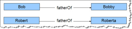
First we have to set up the data. We begin by generating four URIs for the new resources.

    ## Create URIs for Bob and Robert (and kids) 
    robert = conn.createURI("http://example.org/people/robert")
	roberta = conn.createURI("http://example.org/people/roberta")
	bob = conn.createURI("http://example.org/people/bob")
	bobby = conn.createURI("http://example.org/people/bobby")

    ## create name and child predicates, and Person class.
    name = conn.createURI("http://example.org/ontology/name")
    fatherOf = conn.createURI("http://example.org/ontology/fatherOf")
    person = conn.createURI("http://example.org/ontology/Person")

    ## create literal values for names    
    bobsName = conn.createLiteral("Bob")
    bobbysName = conn.createLiteral("Bobby")
    robertsName = conn.createLiteral("Robert")
    robertasName = conn.createLiteral("Roberta")

Robert, Bob and the children are all instances of class Person.  It is good practice to identify all resources by an rdf:type link to a class.

    ## Robert, Bob, and children are people
    conn.add(robert, RDF.TYPE, person)
    conn.add(roberta, RDF.TYPE, person)
    conn.add(bob, RDF.TYPE, person)
    conn.add(bobby, RDF.TYPE, person)

    ## They all have names.
    conn.add(robert, name, robertsName)
    conn.add(roberta, name, robertasName)
    conn.add(bob, name, bobsName)
    conn.add(bobby, name, bobbysName)

    ## robert has a child
    conn.add(robert, fatherOf, roberta)
    ## bob has a child
    conn.add(bob, fatherOf, bobby)

SameAs

Now that the basic resources and relations are in place, we'll seed the triple store with a statement that "Robert is the same as Bob," using the owl:sameAs predicate.  The AllegroGraph inference engine recognizes the semantics of owl:sameAs, and automatically infers that Bob and Robert share the same attributes.  Each of them originally had one child.  When inference is turned on, however, they each have two children. 

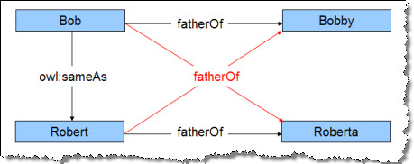
Note that SaveAs does not combine the two resources.  Instead it links each of the two resources to all of the combined children.  The red links in the image are "inferred" triples.  They have been deduced to be true, but are not actually present in the triple store.

This is the critical link that tells the inference engine to regard Bob and Robert as the same resource.

    ## Bob is the same person as Robert
    conn.add(bob, OWL.SAMEAS, robert)

    print "Children of Robert, inference OFF"
    for s in conn.getStatements(robert, fatherOf, None, None): print s   

The search returns one triple, which is the link from Robert to his direct child, Roberta.

Children of Robert, inference OFF
(<http://example.org/people/robert>, <http://example.org/ontology/fatherOf>, <http://example.org/people/roberta>)

This is a getStatements() search with inference turned ON.  This time we added the fifth parameter, True, to getStatements(). This turns on the inference engine.

    print "Children of Robert, inference ON"
    for s in conn.getStatements(robert, fatherOf, None, None, True): print s  

Children of Robert, inference ON
(<http://example.org/people/robert>, <http://example.org/ontology/fatherOF>, <http://example.org/people/roberta>)
(<http://example.org/people/robert>, <http://example.org/ontology/fatherOf>, <http://example.org/people/bobby>)

Note that with inference ON, Robert suddenly has two children because Bob's child has been included.  Also note that the final triple (robert hasChild bobby) has been inferred.  The inference engine has determined that this triple logically must be true, even though it does not appear in the repository.

InverseOf

We can reuse the Robert family tree to see how the inference engine can deduce the presence of inverse relationships.

Up to this point in this tutorial, we have created new predicates simply by creating a URI and using it in the predicate position of a triple.  This time we need to create a predicate resource so we can set an attribute of that resource.  We're going to declare that the hasFather predicate is the owl:inverseOf the existing fatherOf predicate.

The first step is to remove the owl:sameAs link, because we are done with it.

    conn.remove(bob, OWL.SAMEAS, robert)

We'll need a new URI for the hasFather predicate:

    hasFather = conn.createURI("http://example.org/ontology/hasFather")

This is the line where we create a predicate resource.  It is just a triple that describes a property of the predicate.  The hasFather predicate is the inverse of the fatherOf predicate:

     conn.add(hasFather, OWL.INVERSEOF, fatherOf)

First, we'll search for hasFather triples, leaving inference OFF to show that there are no such triples in the repository:

    print "People with fathers, inference OFF"
    for s in conn.getStatements(None, hasFather, None, None): print s    

People with fathers, inference OFF

Now we'll turn inference ON.  This time, the AllegroGraph inference engine discovers two "new" hasFather triples.

    print "People with fathers, inference ON"
    for s in conn.getStatements(None, hasFather, None, None, True): print s  

People with fathers, inference ON
(<http://example.org/people/bobby>, <http://example.org/ontology/hasFather>, <http://example.org/people/bob>)
(<http://example.org/people/roberta>, <http://example.org/ontology/hasFather>, <http://example.org/people/robert>)

Both of these triples are inferred by the inference engine.

SubPropertyOf

Invoking inference using the rdfs:subPropertyOf predicate lets us "combine" two predicates so they can be searched as one.  For instance, in our Robert/Bob example, we have explicit fatherOf relations.  Suppose there were other resources that used a parentOf relation instead of fatherOf.  By making fatherOf a subproperty of parentOf, we can search for parentOf triples and automatically find the fatherOf triples at the same time.

First we should remove the owl:inverseOf relation from the previous example. We don't have to, but it keeps things simple.

    ## Remove owl:inverseOf property.
    conn.remove(hasFather, OWL.INVERSEOF, fatherOf) 

We'll need a parentOf URI to use as the new predicate.  Then we'll add a triple saying that fatherOf is an rdfs:subPropertyOf the new predicate, parentOf:

    parentOf = conn.createURI("http://example.org/ontology/parentOf")
    conn.add(fatherOf, RDFS.SUBPROPERTYOF, parentOf)

If we now search for parentOf triples with inference OFF, we won't find any. No such triples exist in the repository.

    print "People with parents, inference OFF"
    for s in conn.getStatements(None, parentOf, None, None): print s   

People with parents, inference OFF

With inference ON, however, AllegroGraph infers two new triples:

    print "People with parents, inference ON"
    for s in conn.getStatements(None, parentOf, None, None, True): print s  

People with parents, inference ON
(<http://example.org/people/bob>, <http://example.org/ontology/parentOf>, <http://example.org/people/bobby>)
(<http://example.org/people/robert>, <http://example.org/ontology/parentOf>, <http://example.org/people/roberta>)

The fact that two fatherOf triples exist means that two correponding parentOf triples must be valid.  There they are.

Before setting up the next example, we should clean up:

conn.remove(fatherOf, RDFS.SUBPROPERTYOF, parentOf) 

Domain and Range

When you declare the domain and range of a predicate, the AllegroGraph inference engine can infer the rdf:type of resources found in the subject and object positions of the triple.  For instance, in the triple <subject, fatherOf, object> we know that the subject is always an instance of class Parent, and the object is always an instance of class Child. 

In RDF-speak, we would say that the domain of the fatherOf predicate is rdf:type Parent.  The range of fatherOf is rdf:type Child. 

This lets the inference engine determine the rdf:type of every resource that participates in a fatherOf relationship. 

We'll need two new classes, Parent and Child.  Note that RDF classes are always capitalized, just as predicates are always lowercase.

    parent = conn.createURI("http://example.org/ontology/Parent")
    child = conn.createURI("http://exmaple.org/ontology/Child")

Now we add two triples defining the domain and rage of the fatherOf predicate:

    conn.add(fatherOf, RDFS.DOMAIN, parent)
    conn.add(fatherOf, RDFS.RANGE, child)

Now we'll search for resources of rdf:type Parent.  The inference engine supplies the appropriate triples:

    print "Who are the parents?  Inference ON."
    for s in conn.getStatements(None, RDF.TYPE, parent, None, True): print s

Who are the parents?  Inference ON.
(<http://example.org/people/bob>, <http://www.w3.org/1999/02/22-rdf-syntax-ns#type>, <http://example.org/ontology/Parent>
(<http://example.org/people/robert>, <http://www.w3.org/1999/02/22-rdf-syntax-ns#type>, <http://example.org/ontology/Parent>)

Bob and Robert are parents.  Who are the children?

    print "Who are the children?  Inference ON."
    for s in conn.getStatements(None, RDF.TYPE, child, None, True): print s

Who are the children?  Inference ON.
(<http://example.org/people/bobby>, <http://www.w3.org/1999/02/22-rdf-syntax-ns#type>, <http://exmaple.org/ontology/Child>)
(<http://example.org/people/roberta>, <http://www.w3.org/1999/02/22-rdf-syntax-ns#type>, <http://exmaple.org/ontology/Child>)

Bobby and Roberta are the children. 

Geospatial Search (test20())   Return to Top

AllegroGraph provides the ability to locate resources within a geospatial coordinate system. You can set up either a flat (X,Y Cartesian) or spherical (latitude, longitude) system. The systems are two-dimensional only. (There is no Z or altitude dimension available).

The purpose of the geospatial representation is to efficiently find all entities that are located within a specific circular, rectangular or polygonal area.

Cartesian System

A Cartesian system is a flat (X,Y) plane. Locations are designated by (X,Y) pairs. At this time, AllegroGraph does not support real-world measurement units (km, miles, latitude, etc.,) in the Cartesian system.

The first example uses a Cartesian (X,Y) system that is 100 units square, and contains three people located at various points along the X = Y diagonal.

The example is in the function test20(). After establishing a connection, it begins by creating URIs for the three people.

    exns = "http://example.org/people/"
    conn.setNamespace('ex', exns)
    alice = conn.createURI(exns, "alice")
    bob = conn.createURI(exns, "bob")
    carol = conn.createURI(exns, "carol")

Then we have the connection object generate a rectangualr coordinate system for us to use. A rectangular (Cartesian) system can be used to represent anything that can be plotted using (X,Y) coordinates, such as the location of transistors on a silicon chip.

    conn.createRectangularSystem(scale=10, xMax=100, yMax=100) 

The size of the coordinate system is determined by the xMin, xMax, yMin and yMax parameters. The minimum values default to zero, so this system is 0 to 100 in the X dimension, and 0 to 100 in the Y dimension.

The scale parameter influences how the coordinate data is stored and retrieved, and impacts search performance. The task is to locate the people who are within a specific region. As a rule of thumb, set the scale parameter to approximately the same value as the height (Y-axis) of your typical search region. You can be off by a factor of ten without impacting performance too badly, but if your application will search regions that are orders of magnitude different in size, you'll want to create multiple coordinate systems that are scaled for different sized search regions. In this case, our search region is about 20 units high (Y), and we have set the scale parameter to 10 units. That's close enough.

The next step is to create a "location" predicate and enter the locations of the three people.

    location = conn.createURI(exns, "location")
    conn.add(alice, location, conn.createCoordinate(30,30))
    conn.add(bob, location, conn.createCoordinate(40, 40))
    conn.add(carol, location, conn.createCoordinate(50, 50))  

Note that the coordinate pairs need to be encapsulated in a GeoCoordinate object to facilitate indexing and retrieval, using the connection object's createCoordinate() method.

At this point we have a Cartesian coordinate system containing three entities at specific (X,Y) locations. The next step is to define a search region. The first example is a "box" that is twenty units square, with the upper left corner at position (20, 20). The createBox() method requires parameters for xMin, xMax, yMin, and yMax.

    box1 = conn.createBox(20, 40, 20, 40)  

The problem is to find the people whose locations lie within this box:

Locating the matching entities is remarkably easy to do:

    for r in conn.getStatements(None, location, box1) : print r 

This retrieves all the location triples whose coordinates fall within the box1 region. Here are the resulting triples:

(<http://example.org/people/alice>, <http://example.org/people/location>, 
"+30.000000004656613+30.000000004656613"^^<http://franz.com/ns/allegrograph/3.0/geospatial/cartesian/0.0/100.0/0.0/100.0/1.0>)
(<http://example.org/people/bob>, <http://example.org/people/location>, 
"+39.999999990686774+39.999999990686774"^^<http://franz.com/ns/allegrograph/3.0/geospatial/cartesian/0.0/100.0/0.0/100.0/1.0>) 

AllegroGraph has located Alice and Bob, as expected. Note that Bob was exactly on the corner of the search area, showing that the boundaries are inclusive.

We can also find all objects within a circle with a known center and radius. Circle1 is centered at (35, 35) and has a radius of 10 units.

    circle1 = conn.createCircle(35, 35, radius=10)   

A search within circle1 finds Alice and Bob again:

    for r in conn.getStatements(None, location, circle1) : print r 

(<http://example.org/people/alice>, <http://example.org/people/location>, 
"+30.000000004656613+30.000000004656613"^^<http://franz.com/ns/allegrograph/3.0/geospatial/cartesian/0.0/100.0/0.0/100.0/1.0>)
(<http://example.org/people/bob>, <http://example.org/people/location>, 
"+39.999999990686774+39.999999990686774"^^<http://franz.com/ns/allegrograph/3.0/geospatial/cartesian/0.0/100.0/0.0/100.0/1.0>) 

AllegroGraph can also locate points that lie within an irregular polygon. Just tell AllegroGraph the vertices of the polygon:

    polygon1 = conn.createPolygon([(10,40), (50,10), (35,40), (50,70)]) 

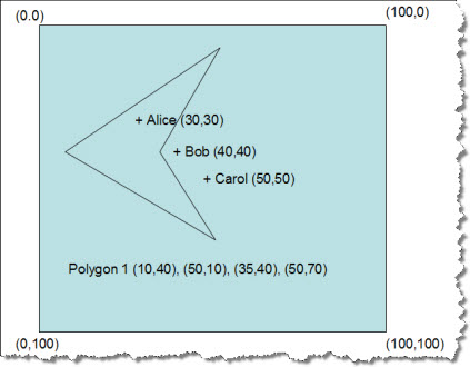
When we ask what people are within polygon1, AllegroGraph finds Alice.

    for r in conn.getStatements(None, location, polygon1) : print r 

(<http://example.org/people/alice>, <http://example.org/people/location>, 
"+30.000000004656613+30.000000004656613"^^<http://franz.com/ns/allegrograph/3.0/geospatial/cartesian/0.0/100.0/0.0/100.0/1.0>)

Spherical System

A spherical coordinate system projects (X,Y) locations on a spherical surface, simulating locations on the surface of the earth. AllegroGraph supports the usual units of latitude and longitude in the spherical system. The default unit of distance is the kilometer (km). (These functions presume that the sphere is the size of the planet earth. For spherical coordinate systems of other sizes, you will have to work with the Lisp radian functions that underlie this interface.)

To establish a global coordinate system, use the connection object's createLatLongSystem() method.

    latLongGeoType = conn.createLatLongSystem(scale=5, unit='degree')

Once again, the scale parameter is an estimate of the size of a typical search area, in the longitudinal direction this time. The default unit is the degree. For this system, we expect a typical search to cover about five degrees in the east-west direction. Actual search regions may be as much as ten times larger or smaller without significantly impacting performance. If the application will use search regions that are significantly larger or smaller, then you will want to create multiple coordinate systems that have been optimized for different scales.

First we set up the resources for the entities within the spherical system. We'll need these subject URIs:

    amsterdam = conn.createURI(exns, "amsterdam")
    london = conn.createURI(exns, "london")
    sanfrancisto = conn.createURI(exns, "sanfrancisco")
    salvador = conn.createURI(exns, "salvador")     

Then we'll need a geolocation predicate to describe the lat/long coordinates of each entity.

    location = conn.createURI(exns, "geolocation")

Now we can create the entities by asserting a geolocation for each one. Note that the coordinates have to be encapsulated in coordinate objects:

    conn.add(amsterdam, location, conn.createCoordinate(52.366665, 4.883333))
    conn.add(london, location, conn.createCoordinate(51.533333, -0.08333333))
    conn.add(sanfrancisto, location, conn.createCoordinate(37.783333, -122.433334)) 
    conn.add(salvador, location, conn.createCoordinate(13.783333, -88.45))  

The coordinates are decimal degrees. Northern latitudes and eastern longitudes are positive.

The next step is to create a box-shaped region, so we can see what entities lie within it.

    box2 = conn.createBox( 25.0, 50.0, -130.0, -70.0) 

This region corresponds roughly to the contiguous United States.

Now we retrieve all the triples located within the search region:

    for r in conn.getStatements(None, location, box2) : print r     

AllegroGraph has located San Francisco:

(<http://example.org/people/sanfrancisco>, <http://example.org/people/geolocation>,
"+374659.49909-1222600.00212"^^<http://franz.com/ns/allegrograph/3.0/geospatial/
spherical/degrees/-180.0/180.0/-90.0/90.0/5.0>) 

This time let's search for entities within 2000 kilometers of Mexico City, which is located at 19.3994 degrees north latitude, -99.08 degrees west longitude.

    circle2 = conn.createCircle(19.3994, -99.08, 2000, unit='km')

    for r in conn.getStatements(None, location, circle2) : print r

(<http://example.org/people/salvador>, <http://example.org/people/geolocation>, 
"+134659.49939-0882700"^^<http://franz.com/ns/allegrograph/3.0/geospatial/spherical/degrees/-180.0/180.0/-90.0/90.0/5.0>)

And AllegroGraph returns the triple representing El Salvador.

In the next example, the search area is a triangle roughly enclosing the United Kingdom:

    polygon2 = conn.createPolygon([(51.0, 2.00),(60.0, -5.0),(48.0,-12.5)])

We ask AllegroGraph to find all entities within this triangle:

    for r in conn.getStatements(None, location, polygon2) : print r 

(<http://example.org/people/london>, <http://example.org/people/geolocation>, 
"+513159.49909-0000459.99970"^^<http://franz.com/ns/allegrograph/3.0/geospatial/spherical/degrees/-180.0/180.0/-90.0/90.0/5.0>)

AllegroGraph returns the location of London, but not the nearby Amsterdam.

Social Network Analysis (test21())   Return to Top

AllegroGraph includes sophisticated algorithms for social-network analysis (SNA). It can examine an RDF graph of relationships among people (or similar entities, such as businesses) and discover:

• Cliques of mutually-supporting individuals.
• The importance of a person within a clique.
• Paths from one individual to another.
• Bottlenecks where information flow might be controlled or break down.

This section has multiple subsections:

• Example Network
• Setting Up the Example
• Creating an Environment
• Creating SNA Generators
• Creating Neighbor Matrices
• Deleting Generators and Matrices
• SNA Search - Ego Group
• SNA Search - Path from A to B
• Graph Measures
• Cliques
• Actor Centrality

Most (but not all) of AllegroGraph's SNA features can be accessed from Python. We access them in multiple ways:

• The Python API to AllegroGraph contains setup functions that let you create an SNA environment ready for queries.
• From Python, we can issue Prolog queries to AllegroGraph. Some of the SNA functions have Prolog equivalents that can be called directly from a query. These are explored in the sections below.
• Within a Prolog query, we can open a window into Lisp and reach for the AllegroGraph's Lisp SNA functions.

Example Network

The example file for this exercise is lesmis.rdf. It contains resources representing 80 characters from Victor Hugo's Les Miserables, a novel about Jean Valjean's search for redemption in 17th-century Paris.

The raw data behind the model measured the strength of relationships by counting the number of book chapters where two characters were both present. The five-volume novel has 365 chapters, so it was possible to create a relationship network that had some interesting features. This is a partial display of the graph in Franz's Gruff graphical browser.

There are four possible relationships between any two characters.

• No direct connection. (They never appeared in the same chapter.) AllegroGraph can locate indirect connections through their mutual acquaintances.
• Barely knows. The characters barely know each other.
• Knows. The two characters appear together in 15 or more chapters.
• Knows well. The two characters appear together in 25 or more chapters.

(The Gruff illustrations were made from a parallel repository in which the resources were altered to display the character's name in the graph node rather than his URI. That file is called lemisNames.rdf.)

Setting Up the Example

The SNA examples are in function test21() in tutorial_examples.py. This exercise begins by borrowing a connection object from an earlier example, and then clearing it so we can start fresh:

    conn = test1();
    conn.clear() 

The next step is to load the lesmis.rdf file and index the triples.

    path1 = "./lesmis.rdf"
    print "Load Les Miserables triples."
    conn.addFile(path1, None, format=RDFFormat.RDFXML);
    conn.indexTriples(all=True)

There are three predicates of interest in the Les Miserables repository. We need to create their URIs and bind them for later use. These are the knows, barely_knows, and knows_well predicates.

    # Create URIs for relationship predicates.
    lmns = "http://www.franz.com/lesmis#"
    conn.setNamespace('lm', lmns)
    knows = conn.createURI(lmns, "knows")
    barely_knows = conn.createURI(lmns, "barely_knows")
    knows_well = conn.createURI(lmns, "knows_well")

We need to bind URIs for two characters: Valjean and Bossuet. Any analysis of Les Miserables will involve Valjean. Bossuet is someone who "barely knows" Valjean, but the two characters are linked through multiple characters who are more strongly connected. We will ask AllegroGraph to find paths from Valjean to Bossuet.

    # Create URIs for some characters.
    valjean = conn.createURI(lmns, "character11")
    bossuet = conn.createURI(lmns, "character64")

Creating an Environment

We're going to use Prolog queries, so we'll need an "environment" for the queries, just like in our example of Prolog rules. The Prolog queries and the SNA generators (below) must reside in the same environment. We also need to set the rule language.

    conn.deleteEnvironment("LesMiserables") ## start fresh 
    conn.createEnvironment("LesMiserables") 
    conn.setEnvironment("LesMiserables") 
    conn.setRuleLanguage(QueryLanguage.PROLOG)

Creating SNA Generators

The SNA functions use "generators" to describe the relationships we want to analyze. A generator encapsulates a list of predicates to use in social network analysis. It also describes the directions in which each predicate is interesting.

In an RDF graph, two resources are linked by a single triple, sometimes called a "resource-valued predicate." This triple has a resource URI in the subject position, and a different one in the object position. For instance:

    (<Cosette>, knows_well, <Valjean>)

This triple is a one-way link unless we tell the generator to treat it as bidirectional. This is frequently necessary in RDF data, where inverse relations are often implied but not explicitly declared as triples.

For this exercise, we will declare three generators:

• "intimates" uses knows_well as a bidirectional predicate.
• "associates" uses knows and knows_well as bidirectional predicates.
• "everyone" uses barely_knows, knows, and knows_well as bidirectional predicates.

"Intimates" takes a narrow view of persons who know one another quite well. "Associates" follows both strong and medium relationships. "Everyone" follows all relationships, even the weak ones. This provides three levels of resolution for our analysis.

In addition, we'll define a dummy generator (emptyGen) just so we can demonstrate how to delete it.

First we'll see how many generators are already in this environment. The connection object's listSNAGenerators() method returns an empty list.

    print "SNA generators known (should be none): '%s'" % (conn.listSNAGenerators())

SNA generators known (should be none): '[]'

The connection object's registerSNAGenerator() method asks for a generator name (any label), and then for one or more predicates of interest. Each predicate should be assigned to the "subjectOf" direction, the "objectOf" direction, or the "undirected" direction (both ways at once). In addition, you may specify a "generator query," which is a Prolog "select" query that lets you be more specific about the links you want to analyze.

"Intimates" follows "knows_well" links only, but it treats them as bidirectional. If Cosette knows Valjean, then we'll assume that Valjean knows Cosette.

    conn.registerSNAGenerator("intimates", subjectOf=None, objectOf=None, 
        undirected=knows_well, generator_query=None)

"Associates" follows "knows" and "knows_well" links.

    conn.registerSNAGenerator("associates", subjectOf=None, objectOf=None, 
        undirected=[knows, knows_well], generator_query=None)

"Everyone" follows all three relationship links.

    conn.registerSNAGenerator("everyone", subjectOf=None, objectOf=None, 
        undirected=[knows, knows_well, barely_knows], 
        generator_query=None)

And one more generator, "emptyGen," that we will use to demonstrate how to delete a generator.

    conn.registerSNAGenerator("emptyGen", subjectOf=None, objectOf=None, undirected=None, generator_query=None)
    print "SNA generators known (should be four): '%s'" % (conn.listSNAGenerators())

When we run this part of the example, the connection object's listSNAGenerators() method detects four generators:

SNA generators known (should be four): '['emptyGen', 'everyone', 'associates', 'intimates']'

Creating Neighbor Matrices

A generator provides a powerful and flexible tool for examining a graph, but it performs repeated queries against the repository in order to extract the subgraph appropriate to your query. If your data is static, the generator will extract the same subgraph each time you use it. It is better to run the generator once and store the results for quick retrieval.

That is the purpose of a "neighbor matrix." This is a persistent, in-memory cache of a generator's output. You can substitute the matrix for the generator in AllegroGraph's SNA functions.

The advantage of using a matrix instead of a generator is a many-fold increase in speed. This benefit is especially visible if you are searching for paths between two nodes in your graph. The exact difference in speed is difficult to estimate because there can be complex trade-offs and scaling issues to consider, but it is easy to try the experiment and observe the effect.

To create a matrix, use the connection object's registerNeighborMatrix() method. You must supply a matrix name (any symbol), the name of the generator, the URI of a resource to serve as the starting point, and a maximum depth. The idea is to place limits on the subgraph so that the search algorithms can operate in a restricted space rather than forcing them to analyze the entire repository.

In the following excerpt, we are creating four matrices to match the four generators we created. In this example, "matrix1" is the matrix for generator "intimates," and so forth.

    print "Neighbor matrices known (should be none): '%s'" % (conn.listNeighborMatrices())
    conn.registerNeighborMatrix("matrix1", "intimates", valjean, max_depth=2)
    conn.registerNeighborMatrix("matrix2", "associates", valjean, max_depth=2)
    conn.registerNeighborMatrix("matrix3", "everyone", valjean, max_depth=2)
    conn.registerNeighborMatrix("emptyMat", "emptyGen", valjean, max_depth=2)

    print "Neighbor matrices known (should be four): '%s'" % (conn.listNeighborMatrices())

Neighbor matrices known (should be none): '[]'
Neighbor matrices known (should be four): '['emptyMat', 'matrix3', 'matrix2', 'matrix1']'

A matrix is a static snapshot of the generator's output. If your data changes, the matrix will need to be rebuilt. For this, use the connection object's rebuildNeighborMatrix() method, and tell it the name of the matrix:

    conn.rebuildNeighborMatrix("matrix1")  
    print "Rebuilt one matrix.  Neighbor matrices known (should be four): '%s'" % (conn.listNeighborMatrices()) 

Rebuilt one matrix.  Neighbor matrices known (should still be four): '['emptyMat', 'matrix3', 'matrix2', 'matrix1']'

Deleting Generators and Matrices

Generators do not occupy much memory, but if your application creates a lot of them it is considered good practice to delete them afterward. Use the connection object's deleteSNAGenerator() method:

    conn.deleteSNAGenerator("emptyGen")
    print "Deleted one generator. SNA generators known: '%s'" % (conn.listSNAGenerators())

Deleted one generator. SNA generators known (should be three): '['everyone', 'associates', 'intimates']'

There is also a deleteNeighborMatrix() method. Unlike generators, matrices occupy significant amounts of memory. Each matrix should be deleted when you are done with it.

    conn.deleteNeighborMatrix("emptyMat")
    print "Deleted one matrix. Neighbor matrices known (should be three): '%s'" % (conn.listNeighborMatrices())

Deleted one matrix. Neighbor matrices known (should be three): '['matrix3', 'matrix2', 'matrix1']'

SNA Search - Ego Group

Our first search will enumerate Valjean's "ego group members." This is the set of nodes (characters) that can be found by following the interesting predicates out from Valjean's node of the graph to some specified depth. We'll use the "associates" generator ("knows" and "knows_well") to specify the predicates, and we'll impose a depth limit of one link. This is the group we expect to find:

The following Python code sends a Prolog query to AllegroGraph and returns the result to Python.

    print "Valjean's ego group (using associates)."
    queryString = """
    (select (?member ?name)
      (ego-group-member !lm:character11 1 associates ?member)
      (q ?member !dc:title ?name))
      """
    tupleQuery = conn.prepareTupleQuery(QueryLanguage.PROLOG, queryString)
    result = tupleQuery.evaluate();
    print "Found %i query results" % len(result)      
    for bindingSet in result:
        p = bindingSet.getValue("member")
        n = bindingSet.getValue("name")
        print "%s %s" % (p, n)

This is the iconic block of code that is repeated in the SNA examples, below, with minor variations in the display of bindingSet values. To save virtual trees, we'll focus more tightly on the Prolog query from this point on:

    (select (?member ?name)
      (ego-group-member !lm:character11 1 associates ?member)
      (q ?member !dc:title ?name))

In this example, ego-group-member is an AllegroGraph SNA function that has been adapted for use in Prolog queries. There is a list of such functions on the AllegroGraph documentation reference page.

The query will execute ego-group-member, using Valjean (character11) as the starting point, following the predicates described in "associates," to a depth of 1 link. It binds each matching node to ?member. Then, for each binding of ?member, the query looks for the member's dc:title triple, and binds the member's ?name. The query returns multiple results, where each result is a (?member ?name) pair. The result object is passed back to Python, where we can iterate over the results and print out their values.

This is the output of the example:

Valjean's ego group (using associates).
Found 8 query results
<http://www.franz.com/lesmis#character27> "Javert"
<http://www.franz.com/lesmis#character24> "MmeThenardier"
<http://www.franz.com/lesmis#character25> "Thenardier"
<http://www.franz.com/lesmis#character28> "Fauchelevent"
<http://www.franz.com/lesmis#character11> "Valjean"
<http://www.franz.com/lesmis#character26> "Cosette"
<http://www.franz.com/lesmis#character23> "Fantine"
<http://www.franz.com/lesmis#character55> "Marius"

If you compare this list with the Gruff-generated image of Valjean's ego group, you'll see that AllegroGraph has found all eight expected nodes. You might be surprised that Valjean is regarded as a member of his own ego group, but that is a logical result of the definition of "ego group." The ego group is the set of all nodes within a certain depth of the starting point, and certainly the starting point must be is a member of that set.

We can perform the same search using a neighbor matrix, simply by substituting "matrix2" for "associates" in the query:

    (select (?member ?name)
      (ego-group-member !lm:character11 1 matrix2 ?member)
      (q ?member !dc:title ?name))

This produces the same set of result nodes, but under the right circumstances the matrix would run a lot faster than the generator.

This variation returns Valjean's ego group as a single list:

    (select ?group
      (ego-group !lm:character11 1 associates ?group))

Valjean's ego group in one list depth 1 (using associates).
"({character27} {character24} {character25} {character28} {character11}
 {character26} {character23} {character55})"

SNA Search - Path from A to B

In the following examples, we explore the graph for the shortest path from Valjean to Bossuet, using the three generators to place restrictions on the quality of the path. These are the relevant paths between these two characters:

Our first query asks AllegroGraph to use intimates to find the shortest possible path between Valjean and Bossuet that is composed entirely of "knows_well" links. Those would be the green arrows in the diagram above. The breadth-first-search-paths function asks for a start node and an end node, a generator, an optional maximum path length, and a variable to bind to the resulting path(s).

    (select ?path
      (breadth-first-search-paths !lm:character11 !lm:character64 intimates 10 ?path))

It is easy to examine the diagram and see that there is no such path. Valjean and Bossuet are not well-acquainted, and do not have any chain of well-acquainted mutual friends. AllegroGraph lets us know that.

Shortest breadth-first path connecting Valjean to Bossuet using intimates.
Found 0 query results

This time we'll broaden the criteria. What is the shortest path from Valjean to Bossuet, using associates? We can follow either "knows_well" or "knows" links across the graph. Those are the green and the blue links in the diagram.

(select ?path
      (breadth-first-search-paths !lm:character11 !lm:character64 associates 10 ?path))

Although there are multiple such paths, there are only two that are "shortest" paths.

Shortest breadth-first path connecting Valjean to Bossuet using associates.
Found 2 query results
"({character11} {character55} {character62} {character64})"
"({character11} {character55} {character58} {character64})"

These are the paths "Valjean > Marius > Enjolras > Bossuet" and "Valjean > Marius > Courfeyrac > Bossuet." AllegroGraph returns two paths because they are of equal length. If one of the paths had been shorter, it would have returned only the short path.

Our third query asks for the shortest path from Valjean to Bossuet using everyone, which means that "barely-knows" links are permitted in addition to "knows" and "knows_well" links.

    (select ?path
      (breadth-first-search-paths !lm:character11 !lm:character64 everyone 10 ?path))

This time AllegroGraph returns a single, short path:

Shortest breadth-first path connecting Valjean to Bossuet using everyone.
Found 1 query results
"({character11} {character64})"

This is the "barely-knows" link directly from from Valjean to Bossuet.

The Prolog select query can also use depth-first-search-paths() and bidirectional-search-paths(). Their syntax is essentially identical to that shown above.

Graph Measures

AllegroGraph provides several utility functions that measure the characteristics of a node, such as the number of connections it has to other nodes, and its importance as a communication path in a clique.

For instance, we can use the nodal-degree function to ask how many nodal neighbors Valjean has, using everyone to catalog all the nodes connected to Valjean by "knows," "barely_knows", and "knows_well" predicates. There are quite a few of them:

The nodal-degree function requires the URI of the target node (Valjean is character11), the generator, and a variable to bind the returned value to.

    print "\nHow many neighbors are around Valjean? (should be 36)."
    queryString = """
    (select ?neighbors
      (nodal-degree !lm:character11 everyone ?neighbors))
      """
    tupleQuery = conn.prepareTupleQuery(QueryLanguage.PROLOG, queryString)
    result = tupleQuery.evaluate();
    for bindingSet in result:
        p = bindingSet.getValue("neighbors")
        print "%s" % (p)
        print "%s" % p.toPython()

Note that this function returns a string that describes an integer, which in its raw form is difficult for Python to use. We convert the raw value to a Python integer using the .toPython() method that is available to all literal values in the Python API to AllegroGraph. This example prints out both the string value and the converted number.

How many neighbors are around Valjean? (should be 36).
"36"^^<http://www.w3.org/2001/XMLSchema#integer>
36

If you want to see the names of these neighbors, you can use either the ego-group-member function described earlier on this page, or the nodal-neighbors function shown below:

    (select (?name)
      (nodal-neighbors !lm:character11 everyone ?member)
      (q ?member !dc:title ?name))

This example enumerates all immediate neighbors of Valjean and returns their names:

Who are Valjean's neighbors? (using everyone).
"Isabeau",  "Labarre",  "Cochepaille",  "Marguerite",  "Babet",  "Woman2",  
"Enjolras",  "Chenildieu",  "Toussaint",  "MmeThenardier",  "Gavroche",  
"Bossuet",  "MotherInnocent",  "Gueulemer",  "Simplice",  "Fauchelevent",  
"MmeMagloire",  "Claquesous",  "Bamatabois",  "Woman1",  "Thenardier",  
"Marius",  "Cosette",  "MlleBaptistine",  "Montparnasse",  "MlleGillenormand",  
"Gervais",  "Brevet",  "Champmathieu",  "Fantine",  "Judge",  "Gillenormand",  
"Javert",  "MmeDeR",  "Scaufflaire",  "Myriel",  

Another descriptive statistic is graph-density, which measures the density of connections within a subgraph.

For instance, this is Valjeans ego group with all associates included.

Only 9 of 28 possible links are in place in this subgraph, so the graph density is 0.32. The following query asks AllegroGraph to calculate this figure for Valjean's ego group:

    (select ?density
      (ego-group !lm:character11 1 associates ?group)
      (graph-density ?group associates ?density))

We used the ego-group function to return a list of Valjean's ego group members, bound to the variable ?group, and then we used ?group to feed that subgraph to the graph-density function. The return value, ?density, came back as a string describing a float, and had to be converted to a Python float using .toPython().

Graph density of Valjean's ego group? (using associates).
"3.2142857e-1"^^<http://www.w3.org/2001/XMLSchema#double>
3.2142857e-1

Cliques

A "clique" is a subgraph where every node is connected to every other node by predicates specified in some generator. AllegroGraph, using everyone ("knows," "knows_well," and "barely_knows"), found that Valjean participates in 239 cliques!

It is counterintuitive that a "clique" should be composed mainly of people who "barely_know" each other, so let's try the same experiment using "associates," which restricts the cliques to people Valjean "knows" or "knows_well." In this case, AllegroGraph returns two cliques. One contains Valjean, Cosette, and Marius. The other contains Valjean and the Thenardiers.

This is the query that finds Valjean's "associates" cliques:

    (select ?clique
      (clique !lm:character11 associates ?clique))

AllegroGraph returns two cliques:

Valjean's cliques? Should be two (using associates).
Number of cliques: 2
"({character11} {character26} {character55})"
"({character11} {character25} {character24})"

The first list is the clique with Marius and Cosette. The second one represents the Thernardier clique.

Actor Centrality

AllegroGraph lets us measure the relative importance of a node in a subgraph using the actor-degree-centrality() function. For instance, it should be obvious that Valjean is very "central" to his own ego group (depth of one link), because he is linked directly too all other links in the subgraph. In that case he is linked to 7 of 7 possible nodes, and his actor-degree-centrality value is 7/7 = 1.

However, we can regenerate Valjean's ego group using a depth of 2. This adds three nodes that are not directly connected to Valjean. How "central" is he then?

In this subgraph, Valjean's actor-degree-centrality is 0.70, meaning that he is connected to 70% of the nodes in the subgraph.

This example asks AllegroGraph to generate the expanded ego group, and then to measure Valjean's actor-degree-centrality:

    (select (?centrality)
      (ego-group !lm:character11 2 associates ?group)
      (actor-degree-centrality !lm:character11 ?group associates ?centrality))

Note that we asked ego-group() to explore to a depth of two links, and then fed its result (?group) to actor-degree-centrality(). This is the output:

Valjean's centrality to his ego group at depth 2 (using associates).
"7.0e-1"^^
7.0e-1

This confirms our expectation that Valjean's actor-degree-centrality should be 0.70 in this circumstance.

We can also measure actor centrality by calculating the average path length from a given node to the other nodes of the subgraph. This is called actor-closeness-centrality. For instance, we can calculate the average path length from Valjean to the ten nodes of his ego group (using associates and depth 2). Then we take the inverse of the average, so that bigger values will be "more central."

The actor-closeness-centrality for Marius is 0.60, showing that Valjean is more central and important to the group than is Marius.

This example calculates Valjean's actor-closeness-centrality for the associates ego group of depth 2.

    (select (?centrality)
      (ego-group !lm:character11 2 associates ?group)
      (actor-closeness-centrality !lm:character11 ?group associates ?centrality))

Valjean's actor-closeness-centrality to his ego group at depth 2 (using associates).
"7.692308e-1"^^<http://www.w3.org/2001/XMLSchema#double>
7.692308e-1

That is the expected value of 0.769.

Another approach to centrality is to count the number of information paths that are "controlled" by a specific node. This is called actor-betweenness-centrality. For instance, there are 45 possible "shortest paths" between pairs of nodes in Valjean's associates depth-2 ego group. Valjean can act as an information valve, potentially cutting off communication on 34 of these 45 paths. Therefore, he controls 75% of the communication in the group.

This example calculates Valjean's actor-betweenness-centrality:

    (select (?centrality)
      (ego-group !lm:character11 2 associates ?group)
      (actor-betweenness-centrality !lm:character11 ?group associates ?centrality))

Valjean's actor-betweenness-centrality to his ego group at depth 2 (using associates).
"7.5555557e-1"^^<http://www.w3.org/2001/XMLSchema#double>
7.5555557e-1

That's the expected result of 0.755.

September 25, 2009